#______________________________Install Packages
install.packages("tidyverse")
install.packages("skimr")
install.packages("janitor")
install.packages("ggplot2")
install.packages("readr")
install.packages("readxl")
install.packages("fixr")        #used by check_for_negative_values
install.packages("gt")          #to create tables
install.packages("webshot2")    #to save table as image
#______________________________Load Packages
library(tidyverse)
library(skimr)
library(janitor)
library(ggplot2)
library(lubridate)
library(stringr)
library(readr)
library(readxl)
library(dplyr)
library(fixr)
library(gt)
library(webshot2)
library(scales)Business Case
A bike-share program that features more than 5,800 bicycles and 600 docking stations. Bikeshare sets itself apart by also offering reclining bikes, hand tricycles, and cargo bikes, making bike-share more inclusive to people with disabilities and riders who can’t use a standard two-wheeled bike. The majority of riders opt for traditional bikes; about 8% of riders use the assistive options. Bikeshare users are more likely to ride for leisure, but about 30% use the bikes to commute to work each day.
In 2016, Bikeshare launched a successful bike-share offering. Since then, the program has grown to a fleet of 5,824 bicycles that are geotracked and locked into a network of 692 stations across Chicago. The bikes can be unlocked from one station and returned to any other station in the system anytime. Until now, Bikeshare’s marketing strategy relied on building general awareness and appealing to broad consumer segments. One approach that helped make these things possible was the flexibility of its pricing plans:
- single-ride passes
- full-day passes and
- annual memberships
Customers who purchase single-ride or full-day passes are referred to as casual riders. Customers who purchase annual memberships are members. Bikeshare’s finance analysts have concluded that annual members are much more profitable than casual riders. Although the pricing flexibility helps Bikeshare tract more customers, Moreno believes that maximizing the number of annual members will be key to future growth.
Rather than creating a marketing campaign that targets all-new customers, Moreno believes there is a solid opportunity to convert casual riders into members. She notes that casual riders are already aware of the Bikeshare program and have chosen Bikeshare for their mobility needs.
Purpose
The director of marketing believes the company’s future success depends on maximizing the number of annual memberships. Therefore, your team wants to understand how casual riders and annual members use Bikeshare bikes differently.
From these insights, your team will design a new marketing strategy to convert casual riders into annual members. But first, Bikeshare executives must approve your recommendations, so they must be backed up with compelling data insights and professional data visualizations.
Moreno has set a clear goal:
Design marketing strategies aimed at converting casual riders into annual members. In order to do that, however, the team needs to know
How do annual members and casual riders use bikes differently?
Why would casual riders buy annual memberships?
How can Bikeshare use digital media to influence casual riders to become members?
Moreno and her team are interested in analyzing the historical bike trip data to identify trends.
Stakeholders
- Lily Moreno: The director of marketing and your manager. Moreno is responsible for the development of campaigns and initiatives to promote the bike-share program.
These may include email, social media, and other channels. - Bikeshare marketing analytics team: A team of data analysts who are responsible for collecting, analyzing, and reporting data that helps guide the marketing strategy.
You joined this team six months ago and have been busy learning about Bikeshare’s mission and business goals—as well as how you, as a junior data analyst, can help Bikeshare achieve them. - The executive team: The notoriously detail-oriented executive team will decide whether to approve the recommended marketing program.
Deliverables
1. A clear statement of the business task
2. A description of all data sources used
3. Documentation of any cleaning or manipulation of data
4. A summary of your analysis
5. Supporting visualizations and key findings
6. Your top three recommendations based on your analysis
Prepare
Data
Bikeshare’s historical trip data is found here: Downloadable here
The data has been made available by Motivate International Inc. under this license.) This is public data that you can use to explore how different customer types are using Bikeshare bikes. But note that data-privacy issues prohibit you from using riders’ personally identifiable information.
Note: if using Posit’s RStudio, use the Divvy 2019 Q1 and Divvy 2020 Q1 datasets. Choosing other data might lead to errors because the data exceeds the memory available in the free plan.
Install Packages
Load Data
#______________________READ Trips from Q1 of 2019 and Q1 of 2020

trips19 <- read_excel("D:/yourdataiq/main/datasets/BikeShareOriginal
                      /Divvy_Trips_2019_Q1.xlsx")
trips20 <- read_excel("D:/yourdataiq/main/datasets/BikeShareOriginal
                      /Divvy_Trips_2020_Q1.xlsx")
Observations
- The two plans offered to casual riders: single-ride passes and full-day passes are not tracked in the data provided all is tracked is whether the user is “Customer” or “Subscriber”.
- The company claims that “Cyclistic users are more likely to ride for leisure, but about 30% use the bikes to commute to work each day”, how is that numbered calculated? nothing in the data shows how it can possibly be calculated!
- UserId is not tracked!? How are we to guess how many users are using the system? This is basic data collection issue which makes the data broad and almost useless.
- Birthyear and gender data is collected which could become helpful if we can figure out how many users we have.
- Up to this point I pretty much know which direction I have to shift my analysis based on what’s provided in the data. This is not bias by any means, it is the simple understanding that the company lacks the knowledge of collecting the right data. It’s like trying to estimate the mpg for a car based on data collected on wiper fluid level.
- At this point I’d have to take my concerns to my manager and advise them of the limitations of the data collected. I will also need to bring up the fact that her hypothesis ” Moreno believes there is a solid opportunity to convert casual riders into members” will be impossible to be justified with this data since we don’t know the exact number of casual and member users.
- Either additional data needs to be provided or the system needs to be adjusted to collect the userId.
- Since the data is provided for Customers and Subscibers as a whole and not broken down to each user I’ll have to see if any
- Column naming took a significant change in 2020 compared to 2019:
- trip_id>ride_id, start_time>started_at, end_time>ended_at,bike_id & tripduration & gender & birthyear were all removed, from_station_id & from_station_name>start_station_name & start_station_id, to_station_id & to_station_name > end_station_id & end_station_name, usertype > member_casual
- end_lat & end_lng & start_lat & start_lng were added
Process
Rename & Type
- Rename columns to make them more relatable and match the other data set
#_____________RENAME 2019 COLUMNS TO MATCH 2020
trips19 <-  rename( trips19,
          ride_id = trip_id,
          started_at = start_time,
          ended_at = end_time,
          rideable_type = bikeid,
          start_station_name = from_station_name,
          start_station_id = from_station_id,
          end_station_name = to_station_name,
          end_station_id = to_station_id,
          member_casual = usertype)
View(trips19)
Set Type
- Change trips19 has ride_id is defined as
"number"while trips20 has it as"char" - Let’s change trips19 to
"char"so it’s easier to analyze after we merge the two data sets together
#_____________CONVERT in trips19: ride_id & rideable_type from num to char
trips19 <- mutate (trips19,
                   ride_id = as.character(ride_id),
                   rideable_type = as.character(rideable_type))
Merge Data Vertically
- Let’s merge the two sets vertically, in other words we want the number of columns to remain the same but the rows to be concatenated (add one set after the other)
- We could use
rbind()but it requires equal number and identical column names. We don’t have that so - We will use
bind_rows()because trips19 has columns that don’t exist in trips20 - trips20 has columns that don’t exist in trips19
#___________COMBINE both datasets vertically via rbind() or bind_rows()
trips19_20 <- bind_rows(trips19, trips20)
Extract Columns
- Let’s take out gender and birthyear from our data
- Both columns are not relevant to this analysis and were not consistent with its collection throughout the dates provided
#________FILTER NEW DATASETS PRIOR TO MANIPULATION - EXCLUDE CERTAIN COLUMNS
trim_trips19_20 <- subset(trips19_20,
                        select = -c( gender, birthyear))

#________OR YOU CAN DO IT THIS WAY AS WELL
trim_trips19_20 <- trips19_20 %>%
                        select(-c( gender, birthyear))
Replace Observations
- Values used in 2019 were not consistent with later values used in 2020
- Later values were adopted and maintained in later years
- We’ll replace 19 values in member_casual column to match those used in later years
#________CLEAN/RENAME member_casual COLUMN FROM member & casual
#________TO Subscriber & Customer
all_trips19_20 <- trim_trips19_20 %>%
          mutate(member_casual = case_when(
                    member_casual == "member" ~ "Subscriber",
                    member_casual == "casual" ~ "Customer",
                    member_casual == "Subscriber" ~ "Subscriber",
                    TRUE ~ "Customer"
          ))
Verify Unique Values
- Let’s make sure there aren’t any values besides the two we thought of
- Any
null, NAor other unexpected values need to be found before we getinto our analysis - Let’s use table() to view how many
uniquemember_casual we have
#________CHECK TO SEE IF ALL WE HAVE ARE THE TWO DESIRED VALUES
table(all_trips19_20$member_casual)

# ___ OUTPUT
Customer Subscriber
  71643     720313
Observations
- My prior observations regarding the data is validated, as we can only gather the total number of rides taken by “Customers” vs “Subscribers”.
- We can break down each type per station, per day, per hour, per gender, per age, but it’s impossible to know how many actual “riders” we are dealing with. How are we supposed to know how many “Customer” users are there?
- How can we even imagine an entire marketing campaign in an attempt to convert users that we can’t quantify?
- The data shows that 9.95% of the trips are taken by Customers!
- Once again, not knowing how many actual users derived all these rides it is not advisable to spend ANY resources trying to analyze nor devise a marketing strategy or campaign to convert any of the 9.95% of our rides.
- My recommendation to my manager that we stop this analysis at this point until additional data is provided, or collection methods are revised.
EDA
Let’s dig around the data for a while, perform some calculations, test a few theories and see if we can discover ideas to pursue.
Drop tripduration
- The information provided does not explain how tripduration was observed - possibly calculated
- I’ll calculate the value based on the strat_at & ended_at values and name it ride_length
- I’ll compare it to the values in tripduration, then I’ll drop tripduration from the data (this is not the original data set)
#________________CALCULATE ride_length AND DROP tripduration

all_trips19_20 <- all_trips19_20 %>%
                mutate(ride_length =
                       as.numeric(difftime(ended_at, started_at, units = 'secs')))

#________________DROP tripduration COLUMN
all_trips19_20 <- all_trips19_20 %>%
                select(-c(tripduration))
Check ride_length
- Let’s dig around in ride_length see if anything sticks out
#___________________CHECK FOR VALUES==0 IN ride_length = 93
any(all_trips19_20$ride_length == 0)
OUTPUT
[1] TRUE


#___________________CHECK how many observations/rows have ride_length=0
sum((all_trips19_20$ride_length == 0))
OUTPUT
[1] 93
Check for NA in ride_length
#___________________CHECK FOR NA VALUES IN ride_length
any(is.na(all_trips19_20$ride_length))
#__________________OF COURSE WE CAN CHECK FOR NON-MISSING DATA (FOR FUN)
any(!is.na(all_trips19_20$ride_length))
OUTPUT
[1] FALSE
Check for ride_length<0
- We’ll make use of package(fixr) and
check_for_negative_values
#___________________CHECK FOR NEGATIVE VALUES IN ride_length
any(all_trips19_20$ride_length < 0)
#___________________ANOTHER WAY IS USING ALL
all(all_trips19_20$ride_length > 0)
OUTPUT
[1] TRUE


#___________________COUNT HOW MANY NEGATIVE ride_length
sum((all_trips19_20$ride_length < 0))
OUTPUT
[1] 117


#______________________IDENTIFY ROWS WITH NEGATIVE ride_length
check_for_negative_values(all_trips19_20$ride_length)
OUTPUT
Data frame contains negative values.
  [1] 520402 648667 651963 652290 653845 655288 655654 656362 657167 658842 660684
663630 663837 664124 664993 667039 669433 669629 669752
 [20] 678262 678499 678889 679182 679252 680301 680757 682576 682662 682853 684254
685564 688888 689153 690765 692831 694009 694476 694635
 [39] 696693 697774 698938 699115 699204 699450 699619 699855 702399 702914 704922
705514 705790 707225 710911 711641 714612 714687 714761
 [58] 715171 715474 719275 719680 725559 726496 730499 731284 731789 736415 737860
738442 740005 740316 740675 742697 743604 743619 745898
 [77] 747194 747233 748686 754006 754853 755032 755536 756753 757832 760822 760913
761163 762641 763241 763358 766631 767985 768102 768693
 [96] 768833 772284 772868 774788 775777 776578 777009 777063 778097 778171 778320
778780 779006 779170 779496 781519 781699 786503 786687
[115] 788671 788946 789252
Rows with negative values
- We can isolate the rows with
ride_length<0by filtering out the location columns
# ___  Rows with ride_length<0
check_for_negative_values(all_trips19_20  |>
                                  select(-c(start_lat, start_lng, end_lat, end_lng))
                                )
OUTPUT
          row col
  [1,] 520402  10
  [2,] 648667  10
  [3,] 651963  10
  [4,] 652290  10
  [5,] 653845  10
  ..
[115,] 788671  10
[116,] 788946  10
[117,] 789252  10
Why ride_length<0
- Let’s extract those 117 rows and see if we can figure out why the
ride_length<0 - Create a dataframe with just the 117 rows and inspect it, maybe something will jump out at us
neg_length <- all_trips19_20[all_trips19_20$ride_length < 0, ]
View(neg_length)
Check for ride_length = 0
- Let’s look at values of 0, maybe there is a relation
zero_length <- all_trips19_20[all_trips19_20$ride_length == 0, ]
dim(zero_length)
OUTPUT
[1] 93 14
Observation
- Well this was easy: all start_station_name & end_station_name are HQ QR
- Let’s see how many times were start_station & end_station_name
= HQ QRandride_length >= 0. The answer is: 675 - After further investigation, it turns out that rows with equal start & end station names were an indication that that specific bike was taken out of circulation for quality control, maintenance or other support related issue, and the system is not setup to allow that information to be entered
- So we need to remove all rows where start & end station names are HQ QR
Check for Dimension
Before dropping the <=0 let’s see the dimensions
dim(all_trips19_20)
OUTPUT
[1] 791956     14
Extract ride_length>0
- We can do this in several ways, I chose to extract the rows ride_length>0
- Then check to see if either the starting or ending station name is HQ QR
- Of course when I mention drop, I actually create a new df with the filtered rows I don’t delete any data
- As you can see, it appears that we have removed 210 rows. And we already know that we had 117 rows with negative values, and 93 rows with zero values. So our math is adding up
- Does that remove all our rows where starting & ending station names are HQ QR?
- Let’s find out
# ___  EXTRACT rows where the ride_length is not negative or zero
all_trips19_20_v2 <- all_trips19_20[all_trips19_20$ride_length > 0, ]
dim(all_trips19_20_v2)
OUTPUT
[1] 791746     14
Check for HQ QR
- Let’s see if HQ QR appears anywhere in the set and if so why?
hq_anywhere <- all_trips19_20_v2 %>%
  filter_all(all_vars(start_station_name == "HQ QR" | end_station_name == "HQ QR"))
dim(hq_anywhere)
OUTPUT
[1] 3558 14- Well, it looks like we still have 3558 rows where they appear and yet the
ride_length >0 - This is one of the times where you have to decide what to do with the 3558 rows (.4%) of the data
- We’ll remove all rows where HQ QR appears in either of the start or end station names
Drop HQ QR rows
- Let’s remove all rows that contain HQ QR in either of their station names
all_trips19_20_v3 <- all_trips19_20_v2[
        !(all_trips19_20_v2$start_station_name == "HQ QR" |
        all_trips19_20_v2$end_station_name == "HQ QR"),]
dim(all_trips19_20_v3)
OUTPUT
[1] 788188     14
Day of Week
- I am shocked that the day of the week was not part of the data breakdown. As that was the first thing I was curious about when I read the case study.
- Let’s see if weekday rides measure up to ones taken on the weekend
- How does the volume vary between weekday and weekend days for high traffic stations
- Those are just a couple of thoughts that would be answered knowing the breakdown of trips taken daily
#____________________ADD TIMEFRAMES_________________________

all_trips19_20_v3 <- all_trips19_20_v3 %>%
  mutate(
    date         = format(as.Date(started_at), format = "%m%d%Y"),     #monthdayYYYY
    year         = format(as.Date(started_at), format = "%Y"),         #Y > 1111 and y > 11
    quarter      = quarters(started_at),                               #quarter
    month        = format(as.Date(started_at), format = "%m"),         #months in number
    day          = day(started_at),                                    #gives the day of the month in number
    day_of_week  = weekdays(started_at),                               #text for the day
  )
Unique Starting Stations
#__________________________LET'S SEE HOW MANY UNIQUE STATIONS WE HAVE
start_id <- all_trips19_20_v3 %>%
  #filter(year == 2020) %>%
  distinct(start_station_id) %>%
  arrange(start_station_id) %>%
  rename(stationID = start_station_id)
dim(start_id)
OUTPUT
[1] 611   1

# ___ If we filter out 2019 we get 606 rows, so 5 stations were removed in 2020
Unique Ending Stations
end_id <-all_trips19_20_v3 %>%
  #filter(year == 2020) %>%
  distinct(end_station_id) %>%
  arrange(end_station_id)  %>%
  rename(stationID = end_station_id)
OUTPUT
[1] 611   1
Compare Starting & Ending
- Let’s compare the two lists of station names: starting & ending lists
- Let’s see if any station acts as an origin and never a destination, and vice versa
identical(start_id$stationID, end_id$stationID)
OUTPUT
[1] FALSE


all.equal(start_id, end_id)
OUTPUT
[1] "Component “stationID”: Mean relative difference: 0.002392677"


glimpse(end_id)
OUTPUT
both are dbl


summary(compare_df_cols_same(start_id, end_id))
OUTPUT
   Mode    TRUE
logical       1


summary(compare_df_cols(start_id, end_id))
OUTPUT
 column_name          start_id            end_id
 Length:1           Length:1           Length:1
 Class :character   Class :character   Class :character
 Mode  :character   Mode  :character   Mode  :character
Outer Join Lists
- In order to get the distinct station IDs from both I’ll outer join the two lists
#__________OUTER JOIN THEM BECAUSE WE WANT ALL DISTINCT STATION ID FROM BOTH
join_station_id <- merge(start_id, end_id, by = 'stationID', all = TRUE)
dim(join_station_id)
OUTPUT
[1] 613   1
Exclude Stations without Coordinates
- Some of the stations don’t appear to have location coordinates
- The plan is to plot all the stations on a map then
- Compare geographical locations and its effects on the number of rides
- Maybe locations in a business district have higher weekday usage while lower weekend numbers
- While other locations that have a higher interest by tourists would have a higher weekend usage
- Maybe locations closer to train stops have higher weekday usage might indicate business commuters taking a train to the city, then using a bike to travel to their job sites
station_coord <- all_trips19_20_v3 %>%
  select( start_station_id,start_lat,start_lng) %>%
  filter(!is.na(start_lat), !is.na(start_lng)) %>%
  group_by(start_station_id, start_lat, start_lng) %>%
  summarize(number_of_rides = n()) %>%
  arrange((start_station_id)) %>%
  rename(stationID = start_station_id)
dim(station_coord)
OUTPUT
[1] 606   4
# ___ We lost some stations because some didn't have geo coordinates
Uncommon Stations
#____________________LETS SEE WHAT WE HAVE UNCOMMON BETWEEN THE TWO
anti_join(join_station_id, station_coord)
# ___ We get the 7 rows in stationID that are not in station_coord
OUTPUT
Joining with `by = join_by(stationID)`
  stationID
1       360
2       361
3       561
4       564
5       565
6       566
7       665
Study The List
- Let’s study the list of 7 stations to see what we might learn
# _____________  LET'S EXTRACT THOSE STATIONS FOR REVIEW
uncommon <- all_trips19_20_v3[all_trips19_20_v3$start_station_id == 360 |
                              all_trips19_20_v3$start_station_id == 361 |
                              all_trips19_20_v3$start_station_id == 561|
                              all_trips19_20_v3$start_station_id == 564|
                              all_trips19_20_v3$start_station_id == 565|
                              all_trips19_20_v3$start_station_id == 566|
                              all_trips19_20_v3$start_station_id == 665, ]
View(uncommon)
OUTPUT
40 ROWS of trips without geolocations, all from 2019.
All rows are for stations that are no longer active in 2020 so we can ignore
Inner Join Lists
- Here I’ll take the cleaned station list and join them with the stations with coordinates.
- Since some in the station list are no longer in use, using inner join will automatically eliminate those unwanted stations from the join_station_id list.
all_active_stations_coord <- inner_join(join_station_id,
                                        station_coord, by ='stationID')

# ____________  DROP NUMBER OF RIDES COLUMN THAT WAS USED TO GROUP THEM
all_active_stations_coord <- all_active_stations_coord %>%
                                 select(-c(number_of_rides))
Save Cleaned File
Now that we cleaned the data to a point where analysis could be performed on it, let’s save it and pass it on to the Data Analysts.
Oh wait, that’s me today.
# __________  SAVE CLEANED DATA
file.create("rcleaned_bikeshare_q1_19_20.csv")
write_csv(all_trips19_20_v3,"rcleaned_bikeshare_q1_19_20.csv")
file.create("rcleaned_bikeshare_geolocation_20.csv")
write_csv(all_active_stations_coord,"rcleaned_bikeshare_geolocation_20.csv")
Analyze
Count rides/user
# _____ We can use table
table(all_trips19_20_v3$member_casual)
# _____  Or use gt()
all_trips19_20_v3|>
        count(member_casual) |>
        gt() |>
        opt_table_outline()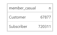
Observations
- I recommend tracking both with IDs so we can narrow in on how many users are more active than others so we can gather some insight on their use
- If users are tracked via ID and zip code, then we’ll know how many of them are business commuters, casual users, or are actual tourists and just use it while in town. This way we can have a more focused marketing campaign.
Summary per User
summary(all_trips19_20_v3$ride_length )
OUTPUT
    Min.  1st Qu.   Median     Mean  3rd Qu.     Max.
1 331 539 1189 912 10632022 - Well that doesn’t do much for me, Let’s group them by user type then summarize
#______________________GROUP BY TYPE OF RIDER THEN CALCULATE STATISTICS
#_____________________AGGREGATE METHOD
all_trips19_20_v3 %>%
  aggregate(ride_length ~ member_casual, mean)

#____________________SUMMARISE & GROUP_BY USER TYPE FOR ALL STATS save as .png
statstable <- all_trips19_20_v3 %>%
  group_by(member_casual) %>%
  summarise(
    max = max(ride_length),
    min = min(ride_length),
    median = median(ride_length),
    mean = round(mean(ride_length), digits = 0)
    ) %>%
  gt()
  gtsave(statstable,"userstats1.png")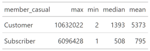
Rides per Year
Total Rides
- Of course everyone always wants to know, how are we doing compared to last year?
- Well let’s see how our total rides performed year after year
#_______________TOTAL TRIPS FROM YEAR TO YEAR
trips_year <- all_trips19_20_v3 %>%
    group_by(year) %>%
    summarise(number_of_rides =n()) %>%
    mutate(pct_change = percent((number_of_rides - lag(number_of_rides))/lag(number_of_rides))) %>%
    gt() %>%
    tab_header(title =md("**Total rides/year_** "))
gtsave( trips_year, "trips_year.png")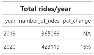
Rides per User/Year
#___________________YEARLY CHANGE PER USER TYPE
user_year <- all_trips19_20_v3 %>%
    group_by(member_casual, year) %>%
    summarise(number_of_rides =n()) %>%
    mutate(pct_change = percent((number_of_rides - lag(number_of_rides))/lag(number_of_rides))) %>%
    gt() %>%
    tab_header(title =md("**Rides/year per user type** "))
gtsave( user_year, "user_per_year.png")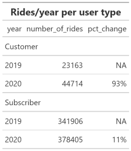
Observations
- The table above clearly shows that marketing has done a great job in attracting new Customers with a 93% increase.
- Actually the Subscriber increase is very good as well
- Once again the disparity between the total of rides by each user type is glaring and looking at the previous table that showed a 16% in total rides from 2019 to 2020, we can conclude that the 93% increase only contributed to 5% of the total rides.
- It is imperative that we tie the number of users to the number of rides (which is not done at this time) to gain any meaningful insight from our analysis
Rides per Day
- Let’s see the breakdown for rides/day/usertype
#_____________USE TABLE FOR BREAKDOWN TOTAL RIDES/DAY/USERTYPE
daily_table <- trips_19_20 %>%
  group_by(member_casual, week_day) %>%
  summarise(max = max(ride_length),
            min = min(ride_length),
            median = median(ride_length),
            mean = round(mean(ride_length), digits = 0),
            number_of_rides =n()) %>%
  gt() %>%
  tab_header(
      title =md("**Daily breakdown for both _user types_** ")
      ) %>%
  fmt_number(columns = c(median,mean), decimals = 0)
gtsave( daily_table,"dailybkdwn3.png")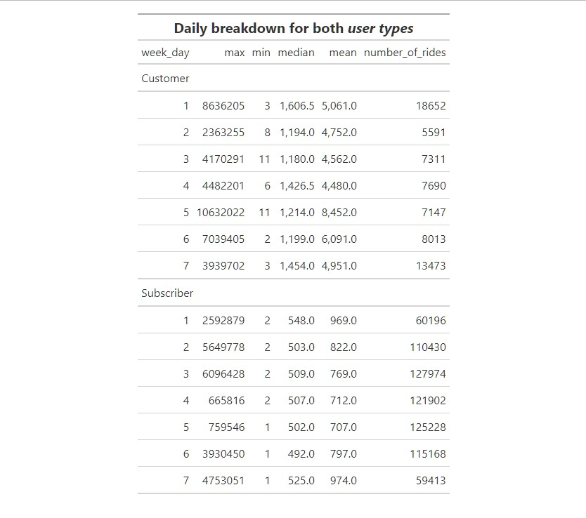
Condensed Table
#________________CONDENSE TABLE FOR EASY READ
condensed_table <- trips_19_20 %>%
  group_by(member_casual, week_day) %>%
  summarise(number_of_rides =n()) %>%
  gt() %>%
  tab_header(title =md("**Daily breakdown for both _user types_** "))
gtsave( condensed_table, "condensed_table.png")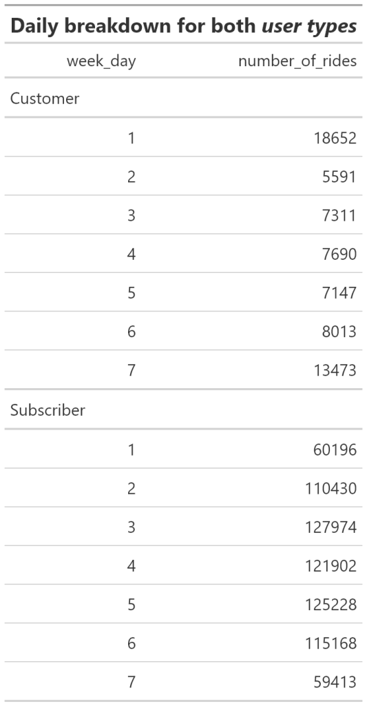
Rides/Day/Year
- Let’s see how the number of rides changed from year to year for every day of the week by user type
#_________________LET'S SEE HOW TRIPS CHANGED PER DAY FROM YEAR TO YEAR
daily_yearly <- trips_19_20 %>%
  group_by(member_casual,year, week_day) %>%
  summarise(number_of_rides =n()) %>%
  gt() %>%
  tab_header(title =md("**Daily breakdown for both _user types year vs year** "))
gtsave( daily_yearly, "daily_yearly.png")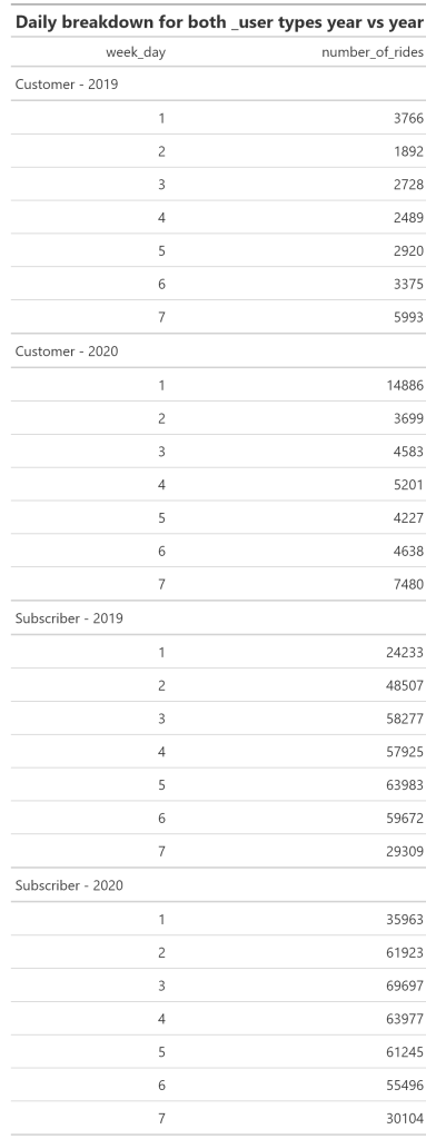
Calculate Percent Change
- How have the rides per day changed over the years
#_________________LET'S SEE PERCENTAGE CHANGE FROM YEAR TO YEAR PER DAY

daily_percent <- trips_19_20 %>%
  group_by(member_casual, week_day, year) %>%
  summarise(number_of_rides =n()) %>%
  mutate(pct_change = percent((number_of_rides - lag(number_of_rides))/lag(number_of_rides))) %>%
  gt() %>%
  tab_header(title =md("**Daily percent change for both _user types year vs year** "))
gtsave( daily_percent, "daily_percent.png")
Observations
FYI day 1 = Sunday, day 2 = Monday and so on
Customers user type:
- Customer users are more active on Saturdays and Sundays which would cause one to believe that those could be tourists or visitors from one of the suburbs of Chicago.
- As I noted before, tracking zip code for users or userId with a profile would quickly focus and clarify our path to a more insightful analyis
- The most obvious percent increase is on day 1 which is Sunday
- Saturday only had a 25% increase but yet still has the second most rides second to Sunday
- I am not sure how you can convert weekend users to Subscribers if they are just visitors that might travel to the city on occasions, not knowing the pricing of a daily pass compared to a yearly subscription I need more information to be able to devise a logical effective marketing strategy for their conversion.
- We also don’t know if any of the users are repeat users or all these are new cyclists that are exposed to our bikes.
- If we are generating unique users it will be worth marketing to them with a different plan than the regular commuters that comprise the weekday usage as shown by the Subcriber type.
Subscriber user type:
- Regardless of which year you review, the weekday use of this type of user overwhelms the weekend numbers
- Thursday and Fridays showed a decline in rides but those numbers are still much higher than weekend numbers
- Cause of these declines could be lack of bikes to use, how do we know how many bikes are at each station?
- How do we know if a user proceeds to their regular station to pick up a bike and realizes none are available?
- Does the app show bikes available at each station at all times?
- Do we track how many times the user had to go to an alternate station due to the lack of availability of bikes?
- Those are numbers that can easily be tracked with a more user friendly app.
- Once again it comes down to UX, how do we know the frustration level of a user if they have to walk several blocks to another station, or worse yet take a cab or walk instead?
Busiest Stations
- Let’s focus on the most used stations and see if we can derive some relationships or insight based on their locations, proximity to city landmark or anything else that might pop out
Most Rides Started
#________________STATIONS WITH THE LARGEST NUMBER OF RIDES STARTED
top_stations <- trips_19_20 %>%
  group_by(start_station_id) %>%
  summarise(number_of_rides =n()) %>%
  arrange(desc(number_of_rides))
Top 5 Stations/Start
#________________TOP 5 STATIONS WHERE RIDES WERE INITIATED
top_5 <- top_stations %>%
  slice(1:5) %>%
  gt() %>%
  tab_header(title =md("**Top 5 STARTING STATIONS** "))
gtsave( top_5, "top5.png")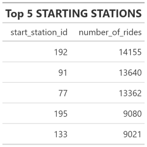
Observations
- Interesting numbers, the top 3 stations individually have about 56% more rides than the 4th busiest station
- I will zoom in on these 3 top stations and see what insight I can gather
Top 3 Percent Change
- As we noticed in the above table, most rides have started in 3 stations
- Let’s see how that changed over the years
#_________________LET'S SEE PERCENTAGE FROM YEAR TO YEAR PER DAY FOR THE TOP STATIONS
rides_top_stations <-trips_19_20 %>%
  filter(start_station_id == 192 | start_station_id ==77 | start_station_id == 91 ) %>%
  group_by(week_day,start_station_id,year) %>%
  summarise(number_of_rides =n()) %>%
  mutate( pct_change = percent((number_of_rides - lag(number_of_rides))/lag(number_of_rides))) %>%
  arrange(desc(start_station_id)) %>%
  gt() %>%
  tab_header(title =md("**Top 3 stations: rides/day year/year** "))
gtsave( rides_top_stations, "rides_top_stations.png")
Observations
- Fist off let me explain how to quickly read the table above:
It is divided in 3 vertical sections
you’ll see in column 1: the number 1 is for day of the week (1=Sunday), the starting station id # 192, then you’ll see two rows for 2019 and 2020, column 2 is number or rides, column3 is percent change from the year before for that same day and same station
- The obvious: weekday numbers 2-6 are more than 10X the weekend day numbers
- Station 192: weekday ride numbers have smaller percent increase from 2019
- Station 91: every day has a decrease in ride numbers except for Sunday with the decreases being significant close to an 20% decrease on average
- Station 77: saw decreases in from Thursday through Saturday with Wednesday having a 1% increase which is not significant
- I’ll dig into the following next to see if it leads somewhere:
There are about 4000 rides per WEEKDAY initiated from just these 3 stations.
Is inventory being tracked at these stations, if so how? If not, are we relying on users to walk to nearby stations?
Proximity of these 3 stations to one another
First thing I worry about: are there enough bikes to rent out from these 3 locations?
Is U/X the cause of the decline in rides?
I will check to see how many rides terminate at these top 3 stations to see if inventory is being replenished by migration from other stations?
I will check to see how many cyclist start and end their rides at these top 3 stations to see if that affects the supply of bikes
Top 3 Stations/2020
#________________DAILY RIDES STARTED FROM THE TOP 3 STATIONS FOR 2020
started_top3 <- trips_19_20 %>%
  filter(start_station_id == 192 | start_station_id ==77 | start_station_id == 91 & year == 2020 ) %>%
  group_by(week_day,start_station_id) %>%
  summarise(number_of_rides =n()) %>%
 # mutate( pct_change = percent((number_of_rides - lag(number_of_rides))/lag(number_of_rides))) %>%
  arrange(desc(start_station_id)) %>%
  gt()%>%
  tab_header(
        title =md("**Top 3 stations: rides/day for 2020** "),
        subtitle = md("STARTING stations")
        )
gtsave( started_top3, "started_top3s.png")
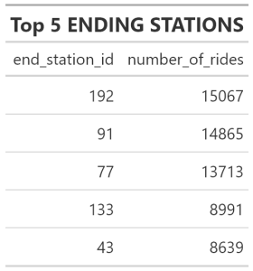
Top 5 Stations/Ending
#__________________  FIGURE OUT TOP ENDING STATIONS
ending_trips<- trips_19_20 %>%
  group_by(end_station_id) %>%
  summarise(number_of_rides =n()) %>%
  arrange(desc(number_of_rides))
#__________________ TOP 5 ENDING STATIONS
end_5 <- ending_trips %>%
  slice(1:5) %>%
  gt() %>%
  tab_header(title =md("**Top 5 ENDING STATIONS** "))
gtsave( end_5, "end5.png")
Rides/Day/User Type
#______________________________GGPLOT WITH _BAR_________________________

trips_19_20 %>%
  group_by(member_casual, week_day) %>%
  summarise(number_of_rides =n())  %>%
  ggplot(aes(x= week_day, y= number_of_rides, fill = member_casual, label = number_of_rides)) +
  geom_bar(stat = "identity") +  #stat="identity" is to tell bar to use y values
  geom_text(size = 3, position = position_stack(vjust = 0.5))+  #positon of bar labels
  labs(title="Total rides per day per user type")
ggsave("ttplot.png")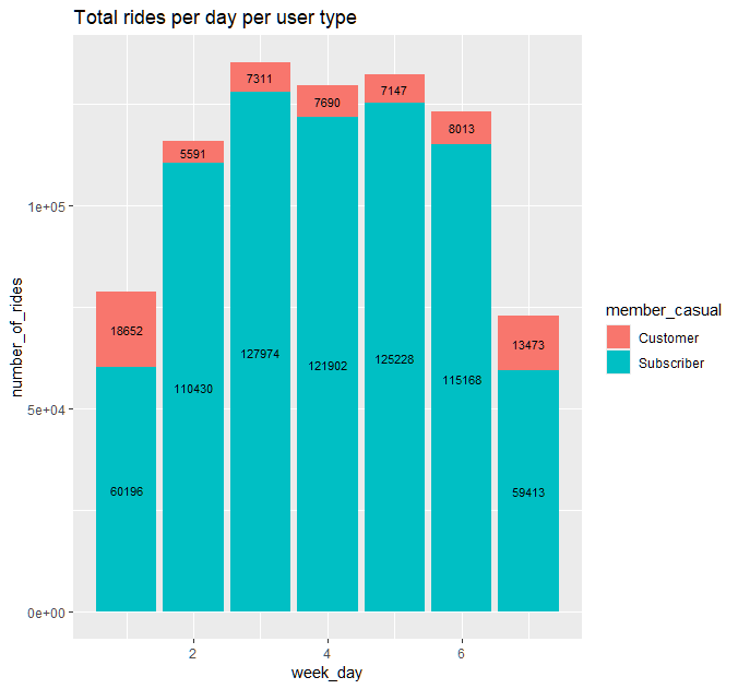
I’ll continue the analysis using SQL and Tableau. For now I’ll list my recommendations:
Recommendations
- Modify the data we track.
- Implement userId so we can focus our analysis and be more insightful.
- Focus on UX at the top stations.
- Stabilize ride numbers at the top stations.
- Reassess the situation in the near future after modifications have been implemented.
TABLEAU
Total Rides per Day
`Rides per Day/Year
- Let’s see what has happened from year to year for the same quarter Q1.
- It appears that the number of rides have gone up for all days EXCEPT Thursday and Fridays, where we see the number of rides have decreased
Rides per Year
Location of Top 5
- Let’s see if the busiest 5 stations are located near a landmark that can help us improve our service
Top 5 Starting Stations - Let’s identify the top 5 performing starting stations
- Maybe the locations can help us understand our users
Interactive Top 5 Graphs
- I’ve gathered multiple top 5 charts together to help me speed up the understanding of the usage
- Just click on the tabs to change views
Top 5 Ending Stations
- I had identified the top 5 starting stations how about we look at the top 5 ending stations
- Maybe this will help us direct our bike availablity or
- Maybe we can better understand our user usage
- Once again I gathered multiple charts together for easier exploration
Top 5 Start=End
- Let’s see if there is a pattern between starting and ending stations - Let’s look how often our user return the bikes to the start station
Observations
- The company claims that “Cyclistic users are more likely to ride for leisure, but about 30% use the bikes to commute to work each day”, how is that numbered calculated?
- The two plans offered to casual riders: single-ride passes and full-day passes are not tracked in the data provided, all we have is user type: “Customer” or “Subscriber”
- The data provided doesn’t link any of the rides to an actual account. Why don’t we track by userId? Don’t Subscribers have to create an account? Why are we just sorting the data by “Member Casual”.
- We can gather more insight if the rideId is linked to a userId, is the data available but not provided for analysis?
- How are docking station locations related to subway, train, or bus stations?
- Are docking stations near parking structures or major tourist, business centers?
- Are users coming to the city via other mode of transportation and using bikes within the city for commuting?
- The objective of the project is to find ways to convert “Customers” to “Subscribers” which is logical except the data provided doesn’t support the theory proposed by Mrs. Moreno. The data shows a large discrepancy between the two users, as Customers account to 9% of Subscribers usage. See table below.
- The data does not show how many actual users are represented by each type. It is illogical to use rideId as userId. The data provided does not promote an insightful analysis regarding the particular hypothesis presented.
- The idea that converting 9% of rides will improve the bottom line, sure but at what cost? How many users are we converting? How many Subscribers do we already have?
- Considering the fact that I am not provided with data relevant to the proposed hypothesis, I would shift my focus on other issues that the data has exposed.
- The facts that weekday ride numbers have been on the decrease for the busiest stations is alarming (see the last table below). The top stations are very close in proximity to one another, so it is possible that users are not getting good service or possibly a competitor has entered the arena and is targeting that specific small area where the top stations are located. Maybe inventory at those stations doesn’t support the volume of rides initiated from there?
- The fact that inventory at those stations is not tracked needs to be addressed.
- The top stations are far more important to the bottom line than wasting resources on the hypothesis that has been proposed, with the data provided. We cannot worry about converting 9% of rides while the top 3 stations are losing rides at a higher pace and by larger numbers than 9%.
Recommendations
- Modify the data we track.
- Implement userId so we can focus our analysis and be more insightful.
- Focus on UX at the top stations.
- Stabilize ride numbers at the top stations.
- Reassess the situation in the near future after modifications have been implemented.
