library(palmerpenguins)
library(dplyr)Sample Data
Packages
R Data
R has built-in data for testing and we’ll cover that first:
- To access the list of default data in R use: data()
- To load the palemerpenguins data set you’ll need to load the package first then you can access it via penguins
- You’ll notice in the code above I only referenced the library(palmerpenguins) but the code will automatically load the corresponding package
Sequences
Vector
x <- c(17, 14, 4, 5, 13, 12, 10)
x
[1] 17 14 4 5 13 12 10#set all elements of this vector that are greater than 10 to be equal 4
x[x > 10] <- 4
x [1] 4 4 4 5 4 4 10#set all elements >= 11 to be equal to 4
x[x>=11] <- 4
x[1] 4 4 4 5 4 4 10Series
Here are some examples of how to generate a series of numbers in R
1:20 [1] 1 2 3 4 5 6 7 8 9 10 11 12 13 14 15 16 17 18 19 20pi:10[1] 3.141593 4.141593 5.141593 6.141593 7.141593 8.141593 9.14159315:1 [1] 15 14 13 12 11 10 9 8 7 6 5 4 3 2 1Sequence
seq(1,20) [1] 1 2 3 4 5 6 7 8 9 10 11 12 13 14 15 16 17 18 19 20incremented
seq(0,10,by=0.5) [1] 0.0 0.5 1.0 1.5 2.0 2.5 3.0 3.5 4.0 4.5 5.0 5.5 6.0 6.5 7.0
[16] 7.5 8.0 8.5 9.0 9.5 10.0by length
seq(5,10,length=30) [1] 5.000000 5.172414 5.344828 5.517241 5.689655 5.862069 6.034483
[8] 6.206897 6.379310 6.551724 6.724138 6.896552 7.068966 7.241379
[15] 7.413793 7.586207 7.758621 7.931034 8.103448 8.275862 8.448276
[22] 8.620690 8.793103 8.965517 9.137931 9.310345 9.482759 9.655172
[29] 9.827586 10.000000along.with
my_seq <- seq(5,10,length=30)
seq(along.with=my_seq)
[1] 1 2 3 4 5 6 7 8 9 10 11 12 13 14 15 16 17 18 19 20 21 22 23 24 25
[26] 26 27 28 29 30seq_along
seq_along(my_seq) [1] 1 2 3 4 5 6 7 8 9 10 11 12 13 14 15 16 17 18 19 20 21 22 23 24 25
[26] 26 27 28 29 30Replicate
If we’re interested in creating a vector that contains 40 zeros, we can use rep(0, times = 40).
rep(0, times=40) [1] 0 0 0 0 0 0 0 0 0 0 0 0 0 0 0 0 0 0 0 0 0 0 0 0 0 0 0 0 0 0 0 0 0 0 0 0 0 0
[39] 0 0If you want a vector of 1000 NAs
z <- rep(NA, 1000)pattern replication
If instead we want our vector to contain 10 repetitions of the vector (0, 1, 2), we can do
rep(c(0,1,2), times=10) [1] 0 1 2 0 1 2 0 1 2 0 1 2 0 1 2 0 1 2 0 1 2 0 1 2 0 1 2 0 1 2design pattern
What if we want to have 0 ten times, 1 10 times, 2 ten times
rep(c(0,1,2),each=10) [1] 0 0 0 0 0 0 0 0 0 0 1 1 1 1 1 1 1 1 1 1 2 2 2 2 2 2 2 2 2 2Sample
- Syntax:
sample(length(x), size, replace, prob) - Let’s select 10 elements at random from these 20 values such that we don’t know how many NAs
sample(c(1,5),10, replace=TRUE) [1] 5 5 1 5 1 1 5 1 1 5dice roll
- Let’s simulate a six-sided dice rolled 4 times.
- Randomly select 4 numbers between 1-6 with replacement which means after selecting a number it is replaced with another random number from the sample
sample(1:6, 4, replace = TRUE)[1] 1 6 2 2without replacement
- In order to sample without replacement, the population size has to be larger than the sample size
- To sample 10 numbers from 1-20 without replacement, means no number appears more than once since we want 10 out of 20
- So the population has to be larger than 10 and it is 20
sample(1:20, 10) [1] 17 9 18 5 10 8 16 13 1 6seed
- Always set the seed so the data can be reproduced and code tested
set.seed(13435)
x <- data.frame("var1"= sample(1:5), "var2"=sample(6:10), "var3"=sample(11:15))
x
var1 var2 var3
1 3 8 14
2 1 7 15
3 5 6 13
4 4 10 12
5 2 9 11shuffle
- All you have to do to shuffle a sample df is to run it again (sample it again)
- Here we’ll resample the five rows and all columns
x <- x[sample(1:5),]
x
var1 var2 var3
5 2 9 11
4 4 10 12
1 3 8 14
2 1 7 15
3 5 6 13insert NAs
- Let’s insert an NA at row 1 & 3 for var2
x$var2[c(1,3)] = NAsubset
- We already know how to subset, so let’s extract all rows from the first column
x[,1][1] 2 4 3 1 5# subset first two rows of all columns
x[1:2,] var1 var2 var3
5 2 NA 11
4 4 10 12# of course to extract the first 2 rows from column3
x[1:2,"var3"][1] 11 12# or
x[1:2,3][1] 11 12probability
- What if we want to simulate a sample of coin flip and want to set the probability to hit 0 at 30% and to hit 1 at 70%
flips <- sample(c(0,1), 100, replace = TRUE, prob = c(0.3, 0.7))
flips
[1] 1 1 0 1 0 1 1 0 1 1 1 1 1 1 1 0 1 0 1 1 1 1 1 1 1 1 1 0 0 1 1 1 1 1 1 1 1
[38] 1 1 0 1 1 1 0 0 1 1 0 1 1 1 1 0 1 0 1 1 1 0 1 1 1 1 1 1 0 0 1 1 1 1 1 1 1
[75] 1 1 1 1 1 1 0 0 1 1 1 0 1 1 1 0 1 1 0 0 1 0 1 0 0 1- Let’s see if the code really held up to what we asked in 70/30
sum(flips)[1] 75letters
- LETTERS is predefined in R.
- If size argument is not defined R outputs the same size as the one you are sampling from
sample(LETTERS) [1] "F" "Q" "I" "M" "A" "J" "S" "N" "V" "P" "W" "C" "H" "R" "X" "L" "Y" "K" "T"
[20] "G" "D" "O" "B" "E" "Z" "U"runif
- runif(number of observations (n), min =0, max = 1)
- generates 20 uniformly distributed random variables between 0 and 1
- you can skip min and max unless you want to set your own values
u <- runif(20)
u
[1] 0.74162842 0.45010751 0.50547285 0.66180244 0.49817421 0.56429714
[7] 0.36579150 0.37193647 0.05800880 0.77295996 0.21509443 0.88119367
[13] 0.22669610 0.56048141 0.23787464 0.01462926 0.87771995 0.93767246
[19] 0.11087709 0.26739988- what if we want values between 0-10 instead
runif(20,0,10) [1] 7.3582436 6.1997381 2.2256081 5.0161484 9.5722421 2.7662729 8.9042757
[8] 2.9351149 6.7219902 0.8150495 4.3802629 6.6191075 4.2666689 9.8145996
[15] 5.9446412 0.9706589 8.5508502 8.7958897 5.2973956 4.7006625Factors
gl
Generates factors by specifying the pattern of their levels. - Syntax: gl(n, k, length= n*k, labels=seq_len(n), ordered = FALSE) - n: integer for the number of levels - k: integer for the number of replications - length: integer giving the length of the result - labels: an optional vector of labels for the resulting factor levels - ordered: logical indicating whether the result should be ordered or not
Examples
- n: number of levels, so if we want to have a vector of values from 1-3 we set n=3
- k: so how many times we want each level replicated before we move to next level. let’s say we set k=2, that means each of the n levels (n=3) will be replicated k times before we move on to the next level.
- So if we have k=2 that means we’ll start with (1 1) that’s 2 replications, then 22 then 33…
- So we will have 11 22 33 11 22 33 so as you see each level (1-3) is replicated 2 times(k=2) till we reach the length we designed in length=20
# for 3 levels and 2 replications
gl(3,2,20)
[1] 1 1 2 2 3 3 1 1 2 2 3 3 1 1 2 2 3 3 1 1
Levels: 1 2 3# for 3 levels and 3 replications
gl(3,3,20) [1] 1 1 1 2 2 2 3 3 3 1 1 1 2 2 2 3 3 3 1 1
Levels: 1 2 3vector & factor
- Define a factor variable and use n=3 (number of levels) k=10(number of replication)
- The length will match the length of x defined below
f <- gl(3,10)
f
[1] 1 1 1 1 1 1 1 1 1 1 2 2 2 2 2 2 2 2 2 2 3 3 3 3 3 3 3 3 3 3
Levels: 1 2 3tapply for mean
- Let’s calculate the mean for each level
- So tapply will take the value of each x at each level and calculate the mean
x <- c(rnorm(10),runif(10),rnorm(10,1))
tapply(x,f,mean)
1 2 3
0.0752080 0.7772303 1.1945657 tapply for range
- Let’s calculate the range of x for each level
tapply(x,f, range)$`1`
[1] -1.438836 1.263505
$`2`
[1] 0.5770678 0.9637785
$`3`
[1] -0.8002445 3.2803129Distributions
R includes a set of random number generators that allow us to simulate from well-know probability distributions, Normal, Poisson, binomial…
For each probability distribution there are typically four functions that start with r, d, p and q, with r the one that actually generates random numbers from that distribution. Here is the breakdown for each:
- d - for density
- r - for random number generation
- p - for cumulative distribution
- q - for quantile function (inverse cumulative distribution)
Normal
The most common probability distribution to work with is the Normal distribution which is the Gaussian distribution. Here is the syntax for norm:
dnorm(x, mean = 0, sd = 1, log = FALSE)
pnorm(q, mean = 0, sd = 1, lower.tail = TRUE, log.p = FALSE)
qnorm(p, mean = 0, sd = 1, lower.tail = TRUE, log.p = FALSE)
rnorm(n, mean = 0, sd = 1)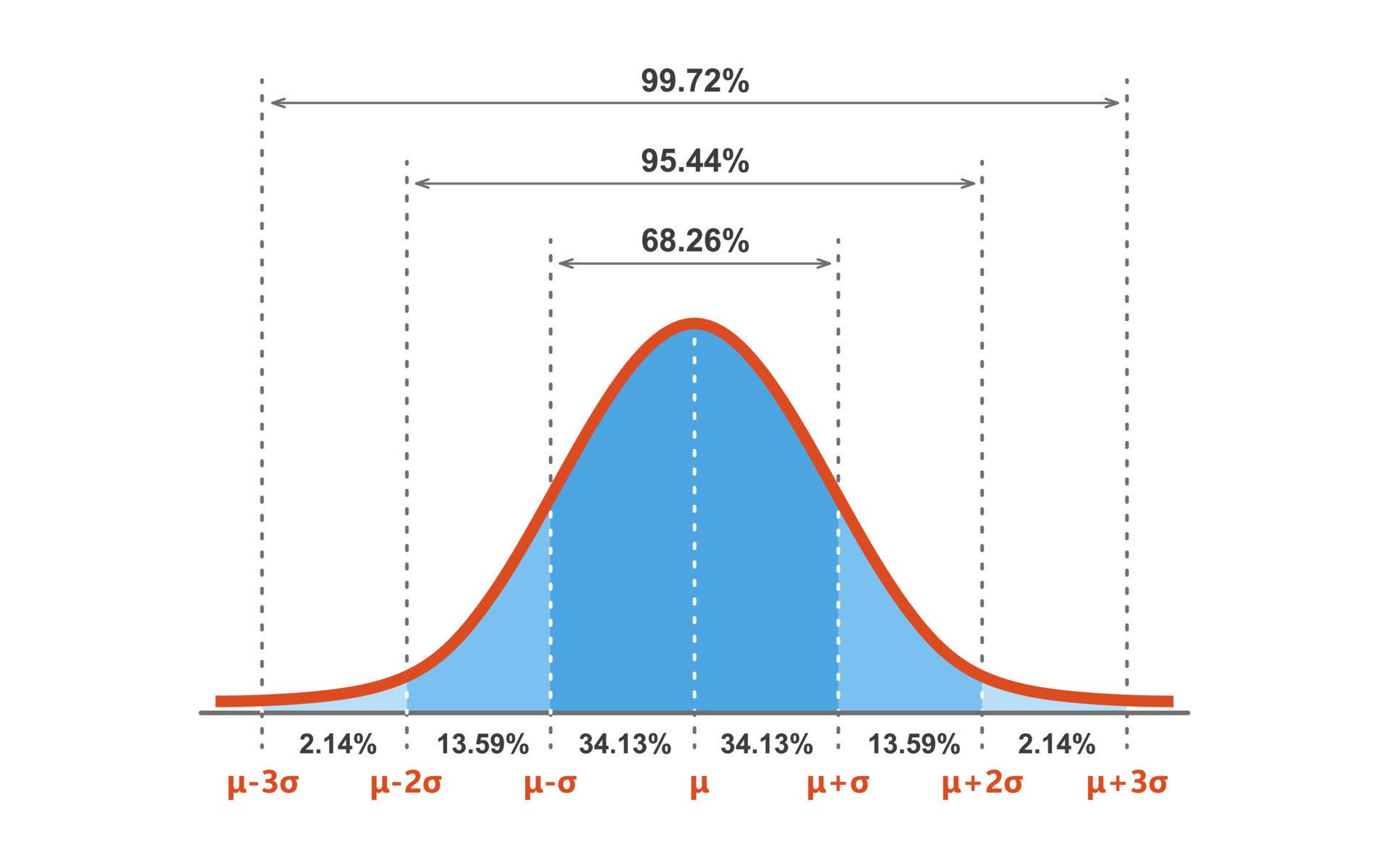 rnorm
rnorm
The rnorm() is used to generate a vector of normally distributed random numbers. - set.seed() is used with conjunction with it so we can reproduce the problem if an error occurs. - Syntax: rnorm(n, mean, sd) - n is the Number of observations (sample size) - mean, is the value of the observation data, default is zero - sd, the standard deviation, default is 1 - If you want to generate random numbers with a custom mean, you can pass it a mean value as the second argument - When you custom the mean it is wise to set.seed that makes it easier to reproduce
# for 10 random numbers from a standard distribution with mean=0 and sd=1
x <- 1:10
y <- rnorm(10)
y
[1] -1.22089371 -1.28474615 -1.12825550 -0.60341370 -0.60276400 -1.66756271
[7] 2.34430392 -0.52450935 -0.01157205 -0.78163359plot(x,y, type="l", lwd=2)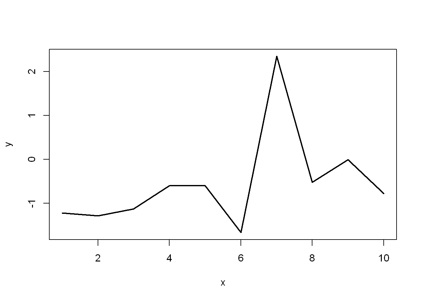
hist(y)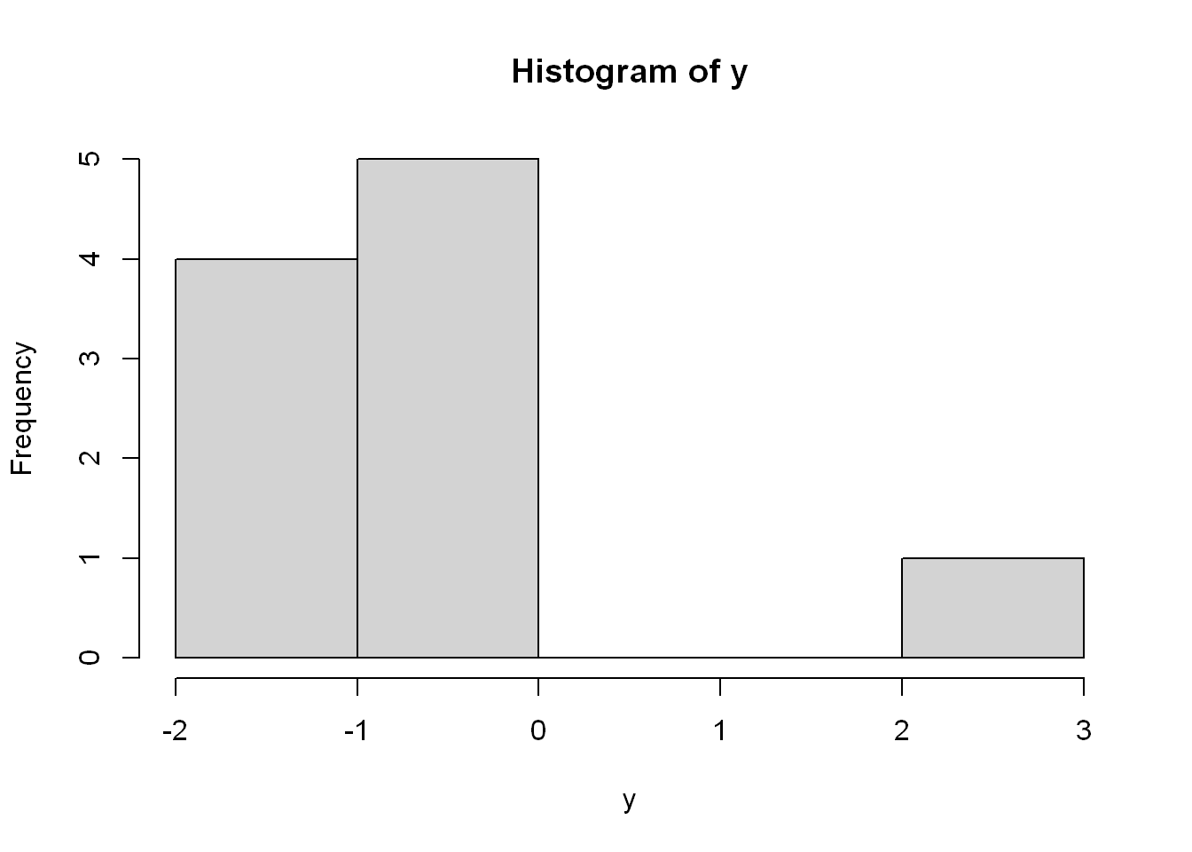
- Let’s repeat it with mean=100 and sd=25
yy <- rnorm(10, 100, 25)
plot(x,yy, type="l", lwd=2)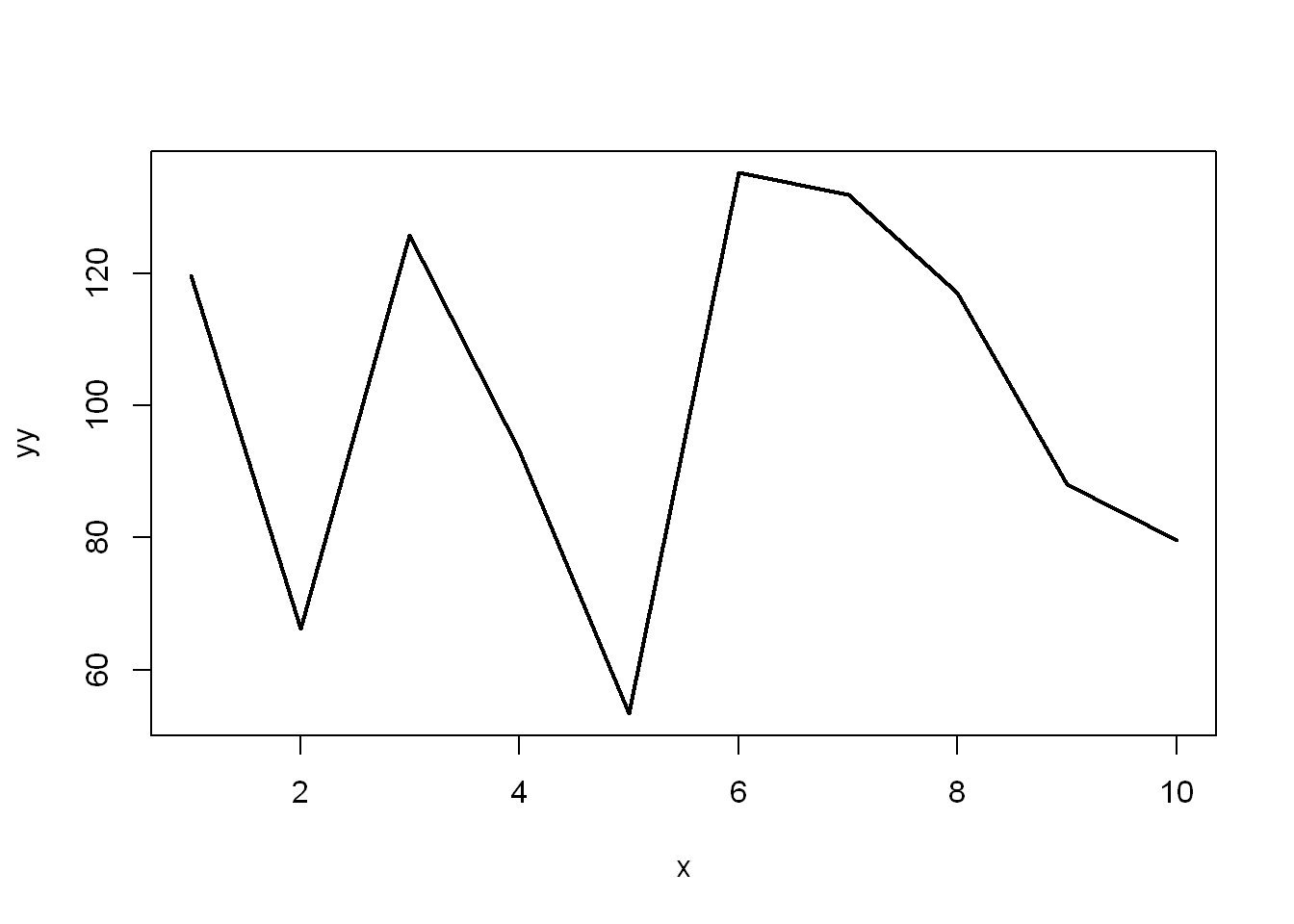
hist(yy)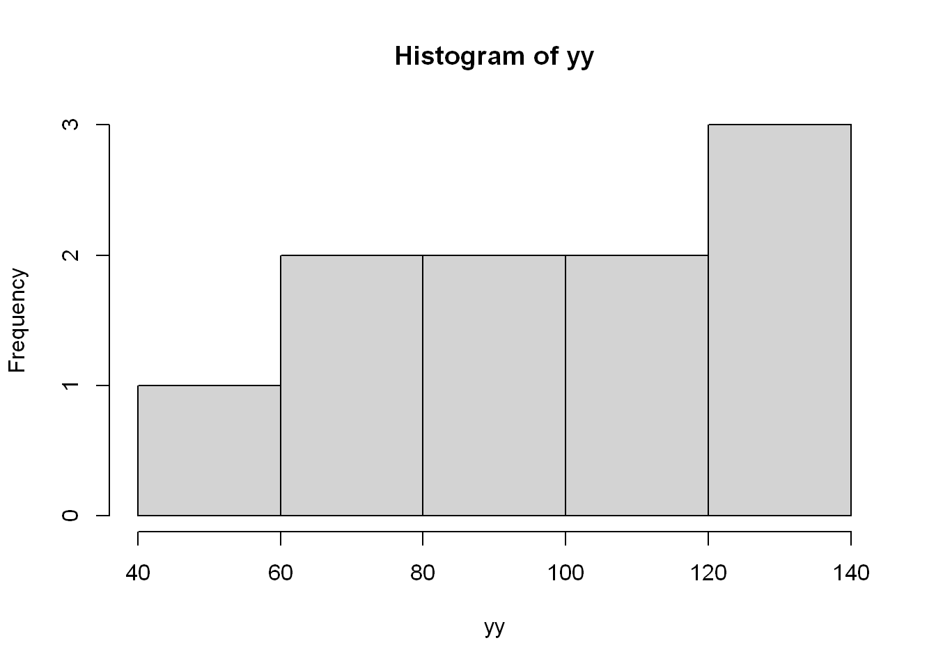
- Let’s repeat it with n=1000 mean=50 and sd=10
- Now you see the shape of the distribution after we draw enough observations
z <- rnorm(1000,50,10)
hist(z)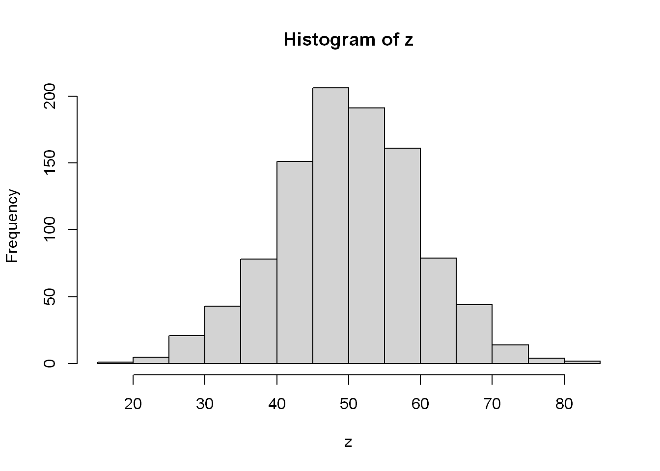
Poisson
A Poisson distribution is a tool that helps to predict the probability of certain events happening when you know how often the event has occurred. It gives us the probability of a given number of events happening in a fixed interval of time.
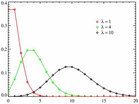
The number of diners in a certain restaurant every day. If the average number of diners for seven days is 500, you can predict the probability of a certain day having more customers.
Because of this application, Poisson distributions are used by businessmen to make forecasts about the number of customers or sales on certain days or seasons of the year. In business, overstocking will sometimes mean losses if the goods are not sold. Likewise, having too few stocks would still mean a lost business opportunity because you were not able to maximize your sales due to a shortage of stock. By using this tool, businessmen are able to estimate the time when demand is unusually higher, so they can purchase more stock. Hotels and restaurants could prepare for an influx of customers, they could hire extra temporary workers in advance, purchase more supplies, or make contingency plans just in case they cannot accommodate their guests coming to the area.
P(x; μ) = (e-μ \* μx) / x!Where:
- The symbol “!” is a factorial.
- μ (the expected number of occurrences) is sometimes written as λ. Sometimes called the event rate or rate parameter.
Example The average number of major storms in your city is 2 per year. What is the probability that exactly 3 storms will hit your city next year?
Step 1: Figure out the components you need to put into the equation. - μ = 2 (average number of storms per year, historically) - x = 3 (the number of storms we think might hit next year) - e = 2.71828 (e is Euler’s number, a constant)
rpois
- Let’s pull 5 random values with mean=10
rpois(5, 10)[1] 7 8 11 7 5replicate
- Let’s replicate the same operation 100 times using replicate
my_pois <- replicate( 100, rpois(5,10))colMeans
- Replicate created a matrix with 100 columns and 5 rows with 5 random numbers.
- Let’s find the mean of each col
cm <- colMeans(my_pois)
cm
hist
- If we plot the histogram
hist(cm)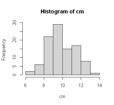
Binomial
The binomial distribution is a discrete probability distribution that calculates the likelihood an event will occur a specific number of times in a set number of opportunities. Use this distribution when you have a binomial random variable. These variables count how often an event occurs within a fixed number of trials. They have only two possible outcomes that are mutually exclusive.
Binomial probability distribution can answer the following questions. What’s the probability of getting: - Six heads when you toss the coin ten times? - 12 women in a sample size of 20? - 3 defective items in a batch of 100? - 2 flu infections in 20 years? This distribution is an example of a Probability Mass Function (PMF) because it calculates likelihoods for discrete random variables. It is an extension of the Bernoulli distribution that can model only 1 trial.
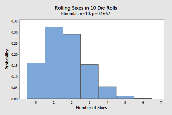
3 sixes in 10 rolls
Suppose you’re playing a game where rolling sixes on a die is really good. You want to know the probability of rolling exactly three sixes in ten die rolls. In this example, - the number of events is x=3 - the number of trials is N = 10 - the probability P is 1/6 = 0.1667
coin flip
- We used the same example in sample above, let’s try it with a binomial distribution here.
- A coin flip is a binary outcome, it’s either 0 or 1 and we are performing 100 trials = N, so let’s use a binomial variable, and we specify the first argument to be 1 = X and we want to see what’s the probability that 1 comes up 70% of the time P=0.7 if we run it 100 times.
- So we want to know how often does 1 come up if we repeat it 100 times if the probability is 70%
rbinom( 1, size = 100, prob = 0.7) [1] 70- If we want to see all the 0’s and 1’s we can request 100 observations of 1 (success) instead of 100 trials like we did above with a prob=0.7 and assign it to a variable
flips2 <- rbinom( 100, size = 1, prob = 0.7)
flips2
[1] 1 1 1 1 1 0 0 0 0 0 1 0 1 0 0 1 1 1 1 1 1 1 0 1 1 1 0 1 0 1 1 0 0 1 1 1 1
[38] 1 0 1 1 1 0 1 1 1 1 0 0 1 0 1 0 1 1 0 0 1 1 0 1 0 0 1 1 1 1 1 1 1 1 1 1 1
[75] 1 1 1 1 0 0 1 0 0 1 1 1 0 1 1 1 1 0 1 0 0 1 1 0 1 1- Let’s see how many times we had
sum(flips2)[1] 67