library(tidyverse)
library(dplyr)
library(lubridate)Fitbit - Reproducible
Data
Packages
Unzip folder
unzip("D:/Education/R/Data/JH_C5_week2/repdata_data_activity.zip",
      exdir= "D:/Education/R/Data/JH_C5_week2/reproducable_walking_data")
Read file
activity <- read.csv("D:/Education/R/Data/JH_C5_week2/reproducable_walking_data/activity.csv")Convert date
First we’ll look at the type of data in each column: it appears date is a “char” so we need to convert
Covert date from “char” to date type
library(lubridate)
str(activity)
'data.frame': 17568 obs. of 3 variables:
$ steps : int NA NA NA NA NA NA NA NA NA NA ...
$ date : chr "2012-10-01" "2012-10-01" "2012-10-01" "2012-10-01" ...
$ interval: int 0 5 10 15 20 25 30 35 40 45 ...activity$date <- ymd(activity$date)Create new columns
wday
- Creating a new column showing the day of the week would help us in the next step
weekend | weekday
Create a new column showing weekdays and weekend days
These will be helpful if we ever need to compare activity levels on weekdays vs weekends or even if we wish to explore a relationship between day of week and activity level
library(dplyr)
activity <- activity |>
        mutate(day_of_week = wday(date, week_start = 1))
# create a weekend variable named weekend
activity <- activity |>
        mutate(weekend = case_when(day_of_week >5 ~ "weekend",
                                        TRUE ~ "weekday"))
CS 1 - Steps per day
The question is a bit vague, do we mean the total number of steps taken per day for each day, or the total number of steps taken per day for the entire dataset?
Well I’ll do both, because I’m curious myself regardless of the intent of the question.
Let’s group the data by date, calculate the total number of steps per day and assign the values to mean_perday
mean_perday now has two columns: date & sum where sum is the total steps taken per day
mean_perday <- activity |>
        group_by(date) |>
        summarise(sum = sum(steps))
Total steps per day
- Now that we have a column of daily total number of steps taken we can simply sum them all together to get the total number of steps taken per day for the entire dataset and assign it to total_steps =570608
total_steps <- sum(mean_perday$sum, na.rm = TRUE)
total_steps
[1] 570608Mean & median
- To calculate the mean and median of the total number of steps taken per day we make use of summary() which will give us the needed answers
- We get a mean=10766 and a median=10765
summary(mean_perday$sum) Min. 1st Qu. Median Mean 3rd Qu. Max. NA's
41 8841 10765 10766 13294 21194 8 Histogram
Plot a histogram for the distribution of total number of steps per day
The magenta line is the mean of the distribution
with(mean_perday, hist(sum, col="green", breaks = 15,
                       main="Total Number of Steps per Day"))
abline(v= mean(mean_perday$sum, na.rm=TRUE), col="magenta",lwd=4)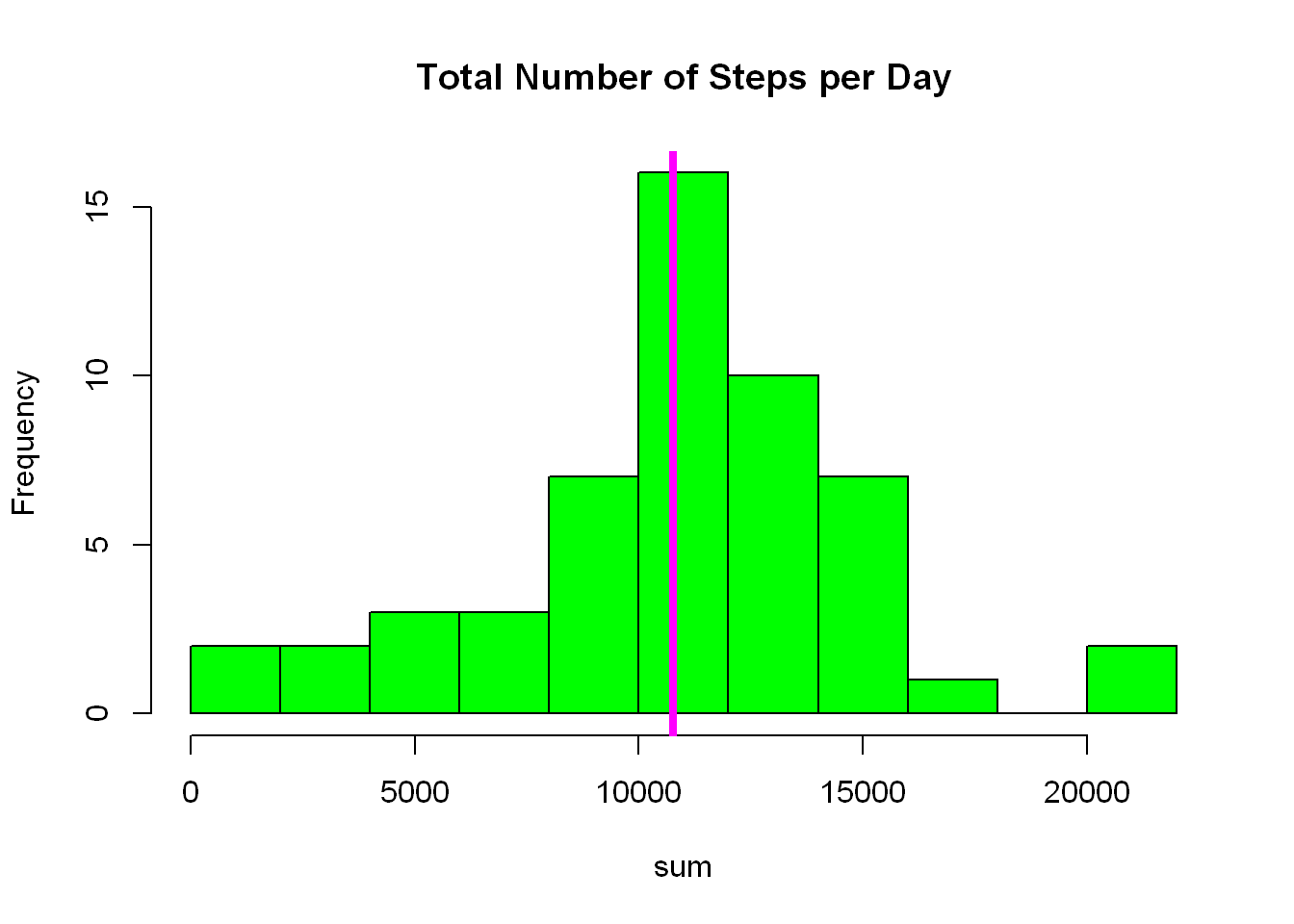
tapply - method 2
#_____________________USING TAPPLY
total.steps <- tapply(activity$steps, activity$date, FUN=sum, na.rm=TRUE)
mean(total.steps,na.rm=TRUE)   #9354.23
[1] 9354.23median(total.steps,na.rm = TRUE) #10395 [1] 10395hist(total.steps, col="green", breaks = 15, main="Total Number of Steps per Day")
abline(v= mean(total.steps,na.rm=TRUE), col="magenta",lwd=4)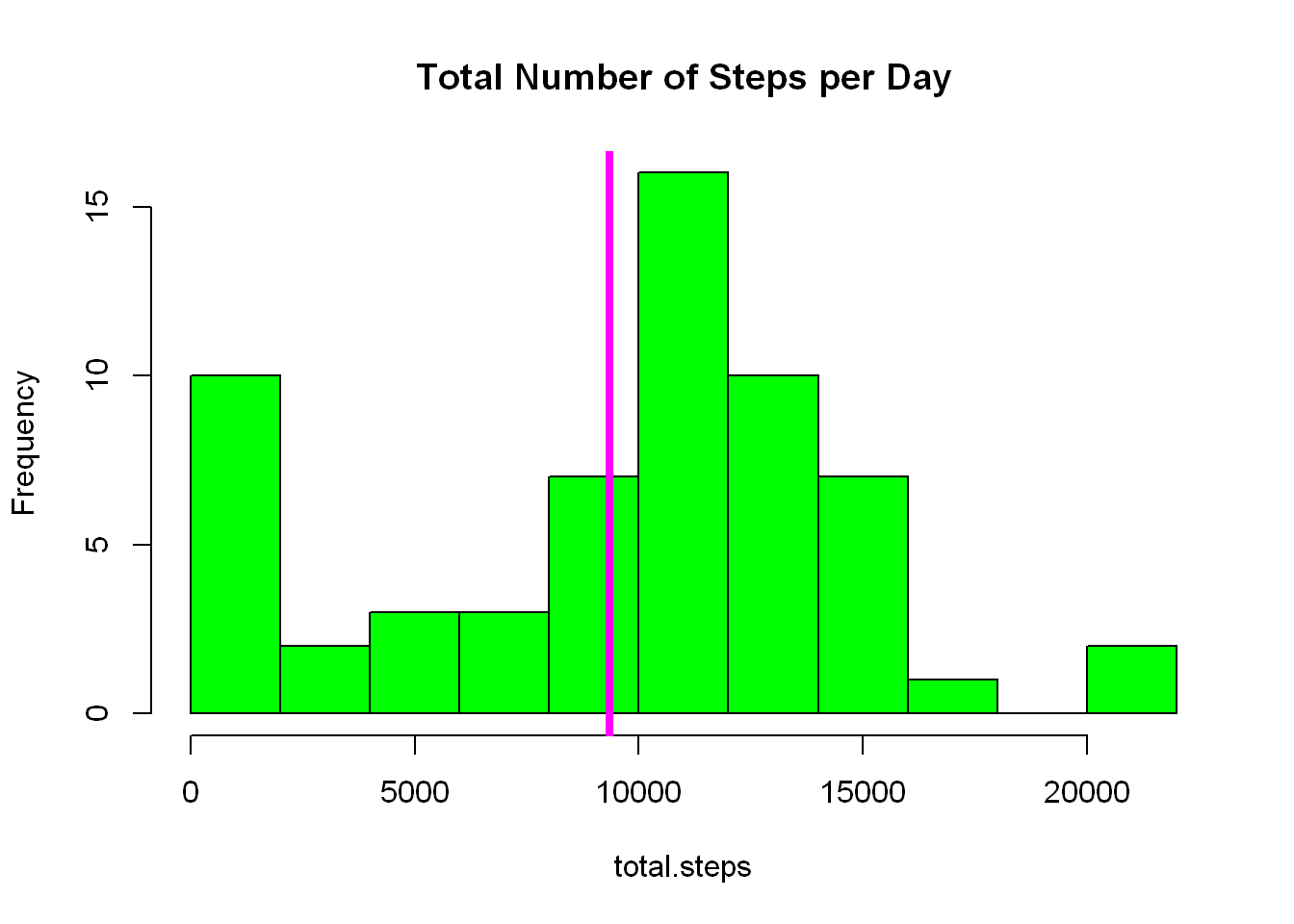
CS 2 - Daily activity
The activity dataset from above shows that each day is divided into 288, 5 minute intervals, in order to look for patterns in daily use it might be wise to compare all the intervals to one another.
In order to do that we’ll calculate the average steps taken for each of the 288 intervals for the entire dataset, and we can do that with the aggregate()
We’ll save the results in activity_perinterval
activity_perinterval <- activity |>
        aggregate(steps~interval, mean)
Time series plot
- Here we’ll plot a time series line graph of the Average Daily Steps per interval to see if any pattern is evident
library(ggplot2)
ggplot(activity_perinterval, aes(interval,steps))+
        geom_line(color="blue") +
        labs(title = "Average Daily Steps per Interval",
             x="Interval", y="Avg Daily Steps")+
        scale_x_continuous(breaks = seq(0,2400, by=240))+
        theme_classic()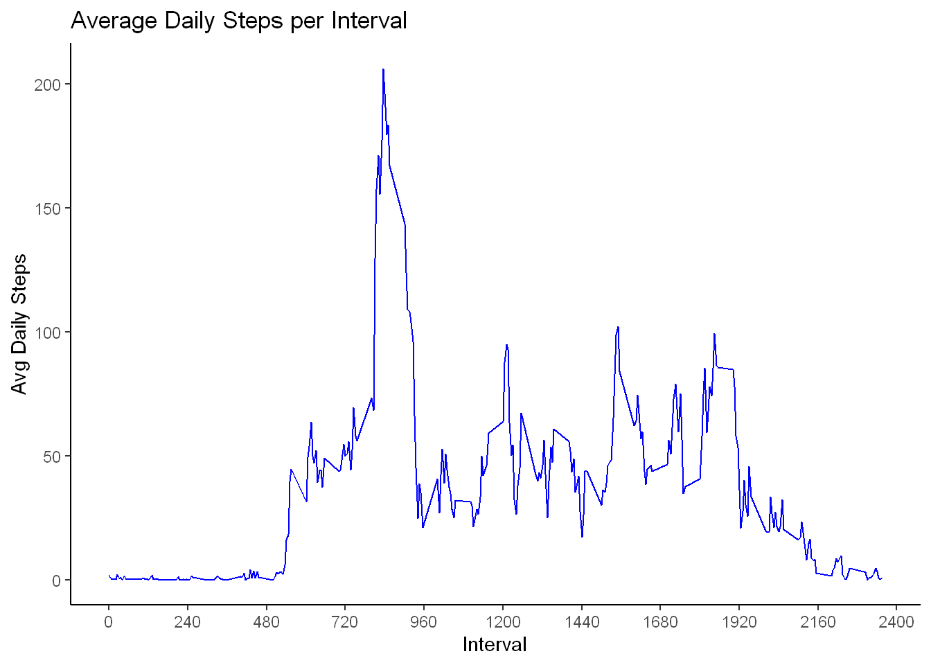
Most active interval
From the plot it is evident that a range of intervals and in particular one interval is by far more popular by the users. To find the exact interval
We can use one line of code as shown below, but let me explain it next:
Let’s start from inside the []: which.max() scans through the steps column and returns the row where the maximum average steps resides
now that we have the row from above, when it’s placed inside the [ , ] it targets that specific row of activity_perinterval
The result shows that row 104 is for interval 835 and has the maximum average steps of 206 per 5 minutes interval
The intervals are setup this way:
First interval is at 0 which is the start of the hour, and increases by 5 every 5 minutes
Once we get to 55 the next increase puts us at the start of the next hour and therefore the interval counter become 100 NOT 60.
So every hours from there the interval counter increases from 100, 200, 300….
So interval 835 would be at 8:35 AM
activity_perinterval[which.max(activity_perinterval$steps),] interval steps
104 835 206.1698CS 3 - Coalesce NAs
Count of NAs
First let’s count how many NA are in the dataset? Total NAs = 2304
Then we find out what percentage of the total rows are NAs (which turns out to be 2.6%)
sum(is.na(activity))[1] 2304mean(is.na(activity))[1] 0.02622951Table option
nas <- is.na(activity)
table(nas)
nas
FALSE TRUE
85536 2304 Replace NAs
Mean of intervals
The plan is to replace each missing NA with the average of that specific interval it is found in.
In order to accomplish that, we need to calculate the mean of every interval for all the days in the dataset
We can accomplish that by using the group_by() and mutate() functions together to create a new column of all the interval means
Save the means in interval_mean
activity_mean <- activity |>
        group_by(interval) |>
        mutate(interval_mean =  mean(steps, na.rm = TRUE))
Coalesce
We go through every row in the df and replace every step which is NA with the mean value for that interval that can be found in the new column interval_mean
We save the new step values in nona_steps
activity_mean$nona_steps <- coalesce(activity_mean$steps, activity_mean$interval_mean) Total steps per day
Just as we did earlier in step 1, we need to calculate the average steps per day now that all the NAs have been replaced with the average for their respective interval.
We can do that just as we did earlier and we just replace with the new df nona_mean_perday
Total steps for all days are: 656737 compared to 570608 before replacing the NAs
nona_mean_perday <- activity_mean |>
        group_by(date) |>
        summarise(sum = sum(nona_steps))
nona_total_steps <- sum(nona_mean_perday$sum)
nona_total_steps
[1] 656737.5Mean & median
To calculate the mean and median of the total number of steps taken per day we make use of summary() which will give us the needed answers
We get a mean= 10766 and median=10766 compared to mean=10766 and median=10765
We shouldn’t have anticipated any major changes since we replace the NAs with the mean of each interval
summary(nona_mean_perday$sum) Min. 1st Qu. Median Mean 3rd Qu. Max.
41 9819 10766 10766 12811 21194 Histogram
Plot a histogram for the distribution of total number of steps per day
The magenta line is the mean of the distribution
with(nona_mean_perday, hist(sum, col="green",
                        breaks = 15, main="Total Number of Steps per Day"))
abline(v= mean(nona_mean_perday$sum, na.rm=TRUE), col="magenta",lwd=4)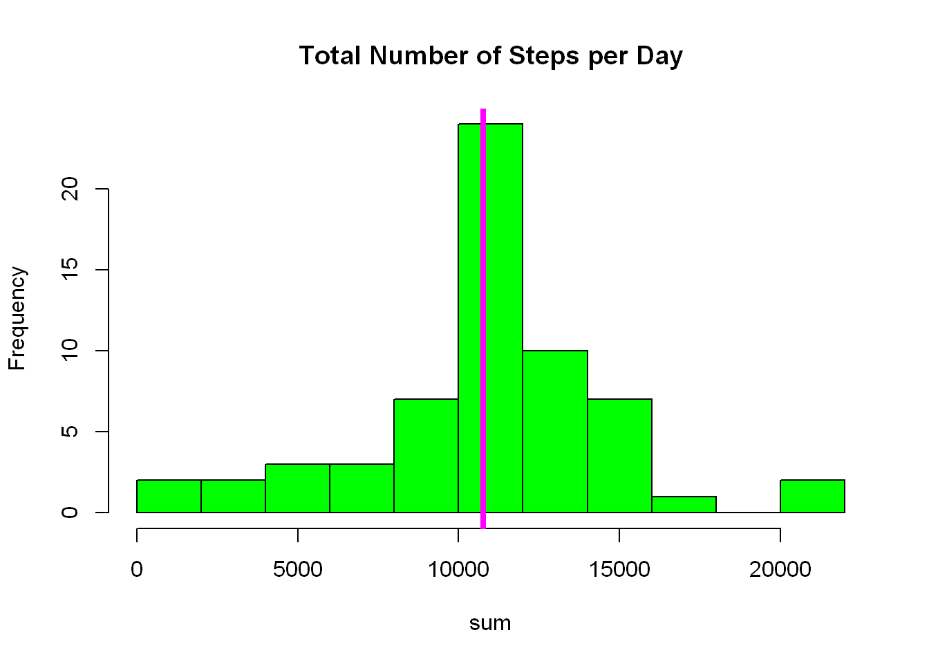
Observation
It might not be glaring but the distribution now is more concentrated around the mean. Look at the frequency count of the tallest bar it is considerably higher than before, and that again is due to replacing all the NAs with mean values.
CS 4 - Weekdays vs Weekends
If you remember when we got started I had created a column named weekend which separates the data by weekday vs weekend days
This comparison becomes fairly simple, all we have to do is aggregate the steps across 2 groups: interval and weekend
Just make sure we use the dataset that included all the repalced NAs activity_mean
Also ensure we use the accurate column that reflects the replaced NAs which would be nona_steps
Load the lattice library since I’ll use lattice for this last plot
library(lattice)
interval_weekday <- activity_mean |>
        aggregate(nona_steps~interval + weekend, mean)
Lattice
xyplot(nona_steps~interval | weekend, interval_weekday,type="l",
       color="blue", xlab = "Interval", ylab = "Average Steps per Interval",
       pch=10, main="Weekend to Weekday Comparison",layout=c(1,2))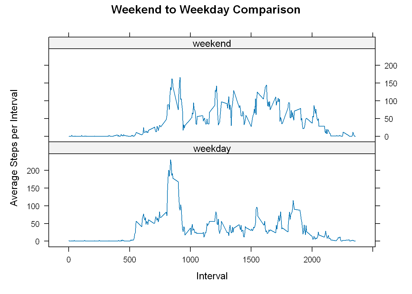
facet_grid
Another option is to use ggplot:
(weekend~.) makes a c(2,1) plot, one over the other
(~weekend) next to each other
ggplot(interval_weekday, aes(interval,nona_steps))+
        geom_line(color="blue") +
        labs(title = "Average Daily Steps per Interval",
             x="Interval", y="Avg Daily Steps")+
        scale_x_continuous(breaks = seq(0,2400, by=240))+
        facet_grid(weekend~.)+
        theme_classic()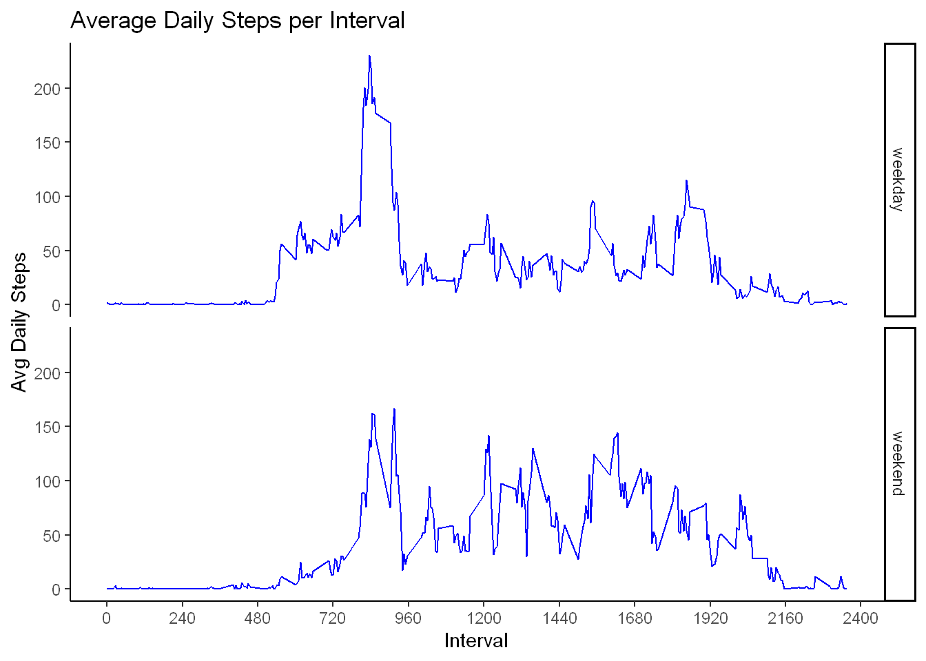
Observation
The visual shows a clear distinction between weekdays activity and weekend days:
On the weekends the activity level is more spread out throughout the day with lower max value.
On the weekdays the activity level is more focused at a certain time of day with a significant spike.
It appears that the users might be professional users that are more active around 8:38 am but then again we have no idea what time zone this data reflects?
Depending on what the business case is there are several possibilities to pursue from this limited data.