if(!file.exists("D:/~/EPConsumption")){dir.create("D:/~/EPConsumption")}

fileUrl <-
"https://d396qusza40orc.cloudfront.net/exdata%2Fdata%2Fhousehold_power_consumption.zip"

download.file(fileUrl,destfile = "D:/~/EPConsumption/zipped.zip", method = "curl")

unzip("D:/~/EPConsumption/zipped.zip", list=TRUE)
#1 household_power_consumption.txt 132960755 2012-10-12 13:38:00

dateDownloaded <- date()
#[1] "Fri Jun 21 09:37:03 2024"

unzip("D:/EPConsumption/zipped.zip",
exdir = "D:/EPConsumption/unzipped")Base - Power EDA 2
Electric Power Consumption
Data
Location
The data can be found at UC Irvine Machine Learning Repository, a popular repository for machine learning datasets. In particular, we will be using the “Individual household electric power consumption Data Set”.
That specific dataset is called Electric Power Consumption and can be downloaded from there as a zip file.
Description
The dataset contains measurements of electric power consumption in one household with a one-minute sampling rate over a period of almost 4 years. Different electrical quantities and some sub-metering values are available. Description of the 9 columns/variables can be found at the UCI web site, I’ll detail them here:
- Date: Date in format dd/mm/yyyy
- Time: time in format hh:mm:ss
- Global_active_power: household global minute-averaged active power (in kilowatt)
- Global_reactive_power: household global minute-averaged reactive power (in kilowatt)
- Voltage: minute-averaged voltage (in volt)
- Global_intensity: household global minute-averaged current intensity (in ampere)
- Sub_metering_1: energy sub-metering No. 1 (in watt-hour of active energy). It corresponds to the kitchen, containing mainly a dishwasher, an oven and a microwave (hot plates are not electric but gas powered).
- Sub_metering_2: energy sub-metering No. 2 (in watt-hour of active energy). It corresponds to the laundry room, containing a washing-machine, a tumble-drier, a refrigerator and a light.
- Sub_metering_3: energy sub-metering No. 3 (in watt-hour of active energy). It corresponds to an electric water-heater and an air-conditioner.
Additional information
This archive contains 2075259 measurements gathered in a house located in Sceaux (7km of Paris, France) between December 2006 and November 2010 (47 months).
The dataset contains some missing values in the measurements (nearly 1,25% of the rows). All calendar timestamps are present in the dataset but for some timestamps, the measurement values are missing: a missing value is represented by the absence of value between two consecutive semi-colon attribute separators. For instance, the dataset shows missing values on April 28, 2007.
Case Study
Examine how household energy usage varies over a 2-day period in February, 2007 by constructing plots using the base plotting system in R
Once you construct the plots, save it to a PNG file with a width of 480px and height of 480px
Name each plot as plot1.png, plot2.png, …
Create a separate R code file named (plot1.R, plot2.R…) that details how you went about constructing the plot. Of course the code should encompass every step from reading the data to saving the output file.
Upload the PNG and R files to the designated Github repository
Here are the 4 plots that need to be constructed, starting with the title, x-axis, y-axis:
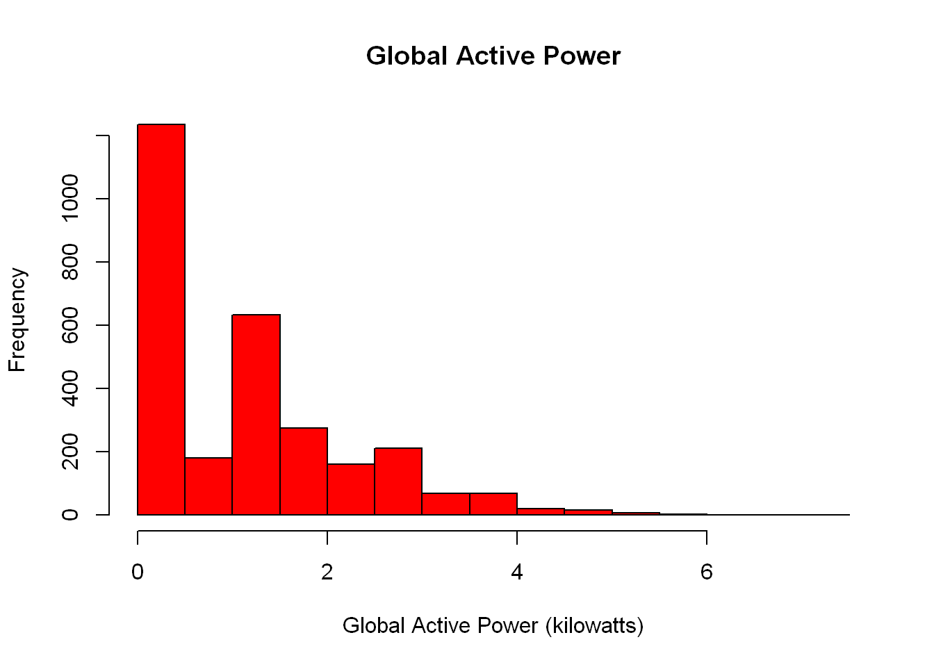
Global Active Power, Global Active Power(kilowatts), Frequency
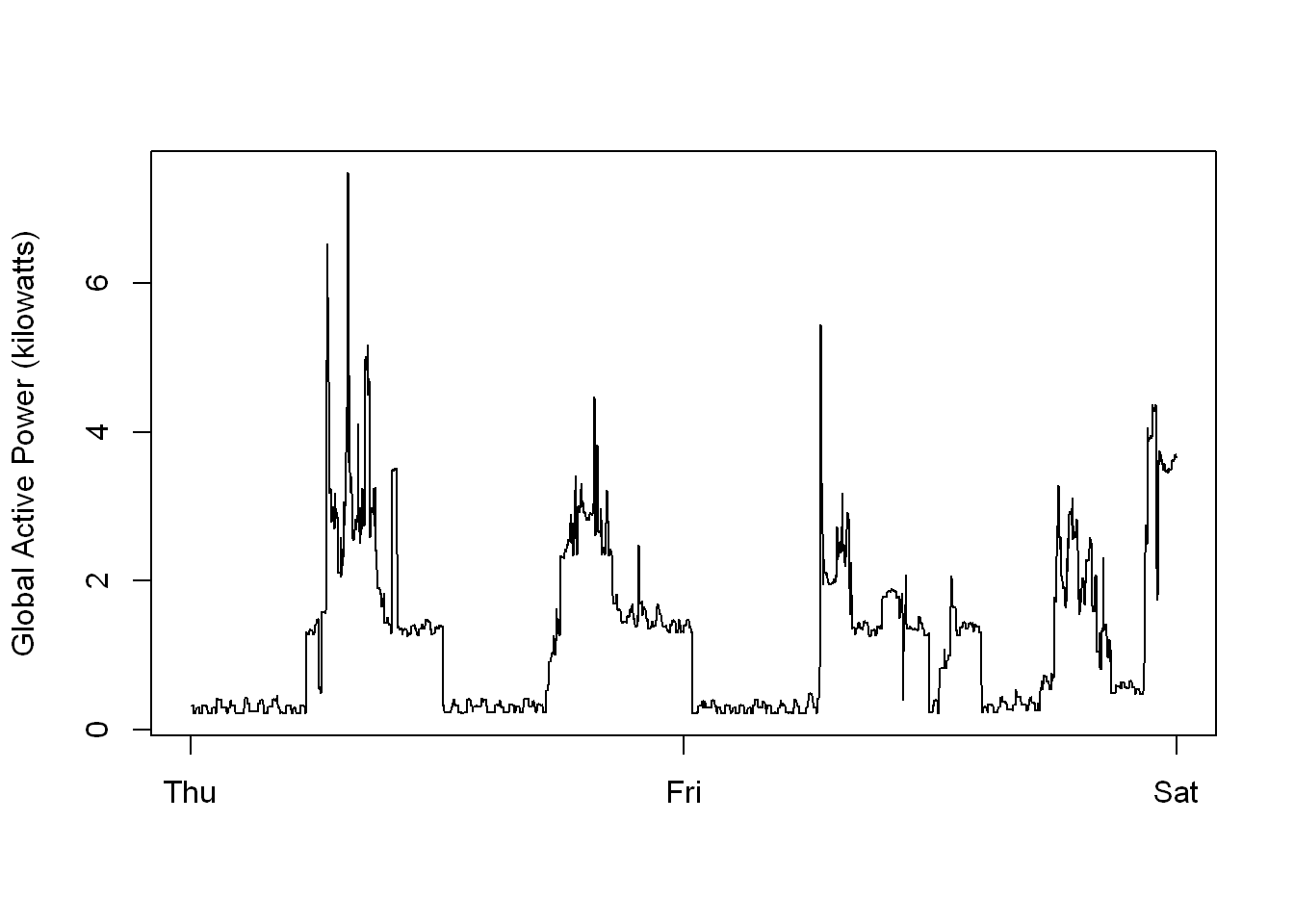
““, Thu-Sat tick marks (no label), Global Active Power(kilowatts)
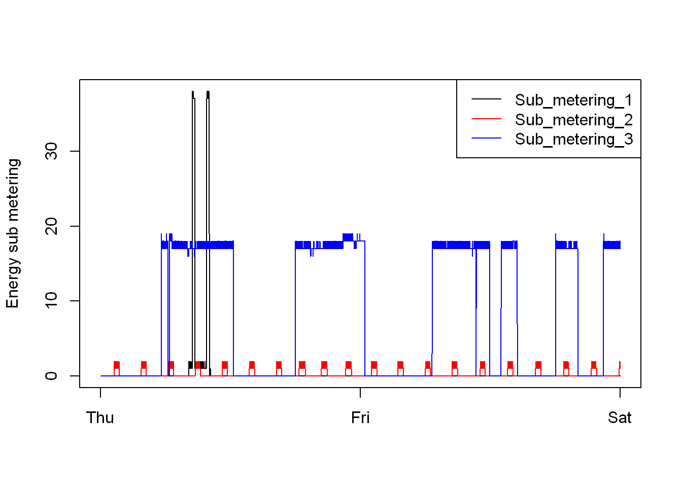
““, Thu-Sat, Energy sub metering, Ledger(Sub_metering_1, Sub_metering_2, Sub_metering_3)
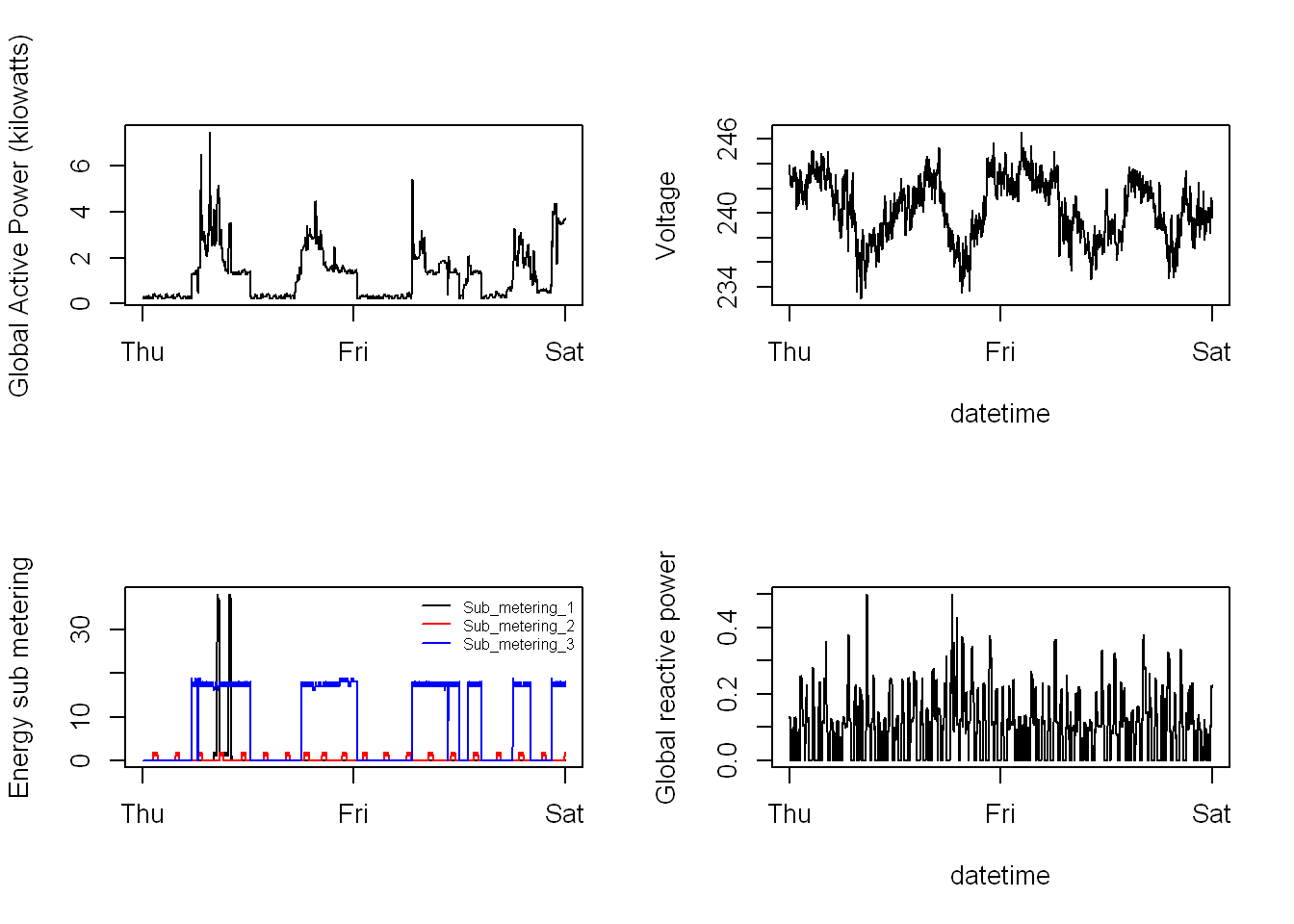
A c(2,2) four graph plot, ““,
Upper left: Thu-Sat=xaxis, Global Active Power=yaxis
Upper right: ““,datetime (Thu-Sat)=xaxis, Voltage=yaxis
Lower left, ““Thu-Sat=xaxis, Energy sub metering=yaxis,Ledger
Lower right: ““,”datetime”Thu-Sat=xaxis,Global_reactive_power=yaxis
Import data
As listed in the description, it’s a large zip file so we’ll download it and list all the files in it to see if the data is broken down into files for each year, each month or whatnot.
Create directory
Let’s check and see if a directory exists before we create it.
Set the location of the file to fileUrl
Download the file to the directory created in step 1
List all the files in the zip folder before we unzip it, hopefully the data is separated into years, months or days so we don’t have to load all the data into R
Well it appears that it contains one zipped file .txt with all the data
Unzip the folder into “unzipped”
                             Name    Length                Date
1 household_power_consumption.txt 132960755 2012-10-12 13:38:00
Warning in unzip("D:/EPConsumption/zipped.zip", exdir =
"D:/EPConsumption/unzipped"): error 1 in extracting from zip fileLoad certain rows
Skip rows
Before we load the entire (over 2 mil. rows) let’s see if we can locate the timeframe that we need from the file. We are looking for 2 days in February 2007, so we’ll eventually load the entire month of February 2007. Remember the date column is formatted dd/mm/yyy
- Setup a connection to our file
- Open the connection
- Read a few rows at a time after skipping several (data starts in Dec. 2006, and we are looking for Feb. 2007)
con <- file("D:/~/EPConsumption/unzipped/household_power_consumption.txt")
open(con)
read.table(con, skip = 400, nrow=2)
Extract data
From the results skipping 400 rows doesn’t even come close, so let’s keep looking. After a few minutes of looking I get close with this subset that I’ll read into datain. The subset starts on 30/1/2007 and ends 6/3/2007 and it’s only 50000 rows as opposed to 2 M.
I’ll filter it further in the next step
con <- file("D:/~/EPConsumption/unzipped/household_power_consumption.txt")
open(con)
header <- read.table(con, nrow=1, sep = ";")
datain <- read.table(con, skip = 65000, nrow=50000, sep = ";")
# we could use the following line but it made no difference
#datain3 <- read.table(con, skip = 65000, nrow=50000, sep = ";", na.strings="?")
close(con)
Clean data
Suppress messages
We’ll use
- lubridate for converting dates and times
- dplyr will be for using mutate()
suppressMessages(library(dplyr))
suppressMessages(library(lubridate))
Extract header
I extracted the header up earlier in the Extract data section.
- I could’ve extracted the header row when I used read.table(header=TRUE)
Set column names
- Assign the header df to colnames of datain
colnames(datain) <- headerTypes
Before we start manipulating the columns, let’s see what all the types are:
str(datain)

'data.frame':   50000 obs. of  9 variables:
        $ Date                 : chr  "30/1/2007" "30/1/2007" "30/1/2007" "30/1/2007" ...
$ Time                 : chr  "20:44:00" "20:45:00" "20:46:00" "20:47:00" ...
$ Global_active_power  : chr  "3.546" "3.510" "3.622" "3.722" ...
$ Global_reactive_power: chr  "0.130" "0.120" "0.120" "0.122" ...
$ Voltage              : chr  "237.410" "236.670" "237.020" "237.950" ...
$ Global_intensity     : chr  "15.000" "14.800" "15.200" "15.600" ...
$ Sub_metering_1       : chr  "2.000" "1.000" "1.000" "1.000" ...
$ Sub_metering_2       : chr  "0.000" "0.000" "0.000" "0.000" ...
$ Sub_metering_3       : num  18 17 17 18 17 17 18 17 17 18 ...
Merge Date & Time
From the case study, I know I will need both the Date and Time columns to be merged and converted so I can use as the x-axis. So let’s
- Merge Date and Time as “char” utilizing the paste()
- Convert the pasted strings using the function dmy_hms and save into a new column datetime
datetime_df <- datain |> mutate(datetime = dmy_hms(paste(Date, Time, sep = " ")))Extract Month
We only need the month of February 2007, according to the case study
feb_datetime <- subset(datetime_df, (month(datetime) == 02))Extract 2 days from February
Since the case study specified 2 days to be Thursday and Friday, and it happens that the first two days in the dataset Feb 1, and Feb 2 are Thursday and Friday, we’ll extract those two days.
twodays <- subset(feb_datetime, (day(datetime) == 01 | day(datetime) == 02) )Extract using %in%
Another way to extract the first two days of February
- Before we merged the Date and Time
- We could use the string values of the Date column and extract the first two days, but we had to have known that the first and second days corresponded to a Thursday and Friday.
- So use this as information only, as I didn’t use this method.
yyy <- datain1[datain1$Date %in% c("2007-02-01","2007-02-02") ,]Convert char to numeric
Since we are planning to plot all the columns, let’s convert them to numeric with:
twodays <- twodays |> mutate(across(Global_active_power:Sub_metering_2, as.numeric))Save to PNG
This is pretty much self-explanatory, just remember that if you save it to a PNG or any other file, it will not be displayed on screen.
png(filename = "/plot1.png", width = 480, height = 480, units = "px")
with(twodays,hist(Global_active_power,
                  xlab="Global Active Power (kilowatts)",
                  main="Global Active Power",
                  col="red") )
dev.off()
Timeseries Plot
Line plot
Relable x-axis
This plot is unique because we relabeled the x-axis
- The case study required labels to be Thursday, Friday and Saturday
- To plot two days only, Thursday & Friday
- Last tick to the right is to be the start of Saturday
- The two days had 2880 rows, whild the three days had 4320 rows
- That means we have 4320 ticks on the x axis and we wanted it divided equally by the tick marks
- Therefore I used 4320/3 for the locations of the tick lables
- Once again I commented out the lines to save the plot to a PNG, all you do is un-comment them
png(filename = "/plot2.png", width = 480, height = 480, units = "px")
plot(twodays$Global_active_power,
                   type = "l",
                   ylab ="Global Active Power (kilowatts)",
                   xlab = "",
                   xaxt="n")
axis(1, at=seq(1,4320, by =4320/3), labels=c("Thu","Fri","Sat"))
#4320 is how many minutes are till end of Saturday. In order to place the last tick
#on the first minute of Sat
#I used the total number of rows for all 3 days 4320 and divided by 3 tick labels
dev.off()
Save to PNG

- Of course you could use the with() to plot as well
- But note when you include the x-axis variable in the plot() then it makes it hard to place the tick marks at the right positions.
- I’ll edit this section when I find a way to attach the tick labels and include both variables in the plot()
with(twodays,plot(Global_active_power,
     type = "l",
     ylab ="Global Active Power (kilowatts)",
     xlab = "",
     xaxt="n"))
# I didn't use this chunk, for information only
Line Plot
Legends
In addition to being a timeseries, this is also a multi-line added as layers on top of the timeseries plot.
- First we plot the timeseries plot
- Then we add line plots with the lines() as layers on top of the first plot
png(filename = "/plot3.png", width = 480, height = 480, units = "px")
plot(twodays$Sub_metering_1,
     type = "l",
     ylab ="Energy sub metering",
     xlab = "",
     col = "black",
     xaxt="n")
axis(1, at=seq(1,4320, by =4320/3), labels=c("Thu","Fri","Sat"))

with(twodays, lines(Sub_metering_2, lty=1, col= "red"))
with(twodays, lines(Sub_metering_3, lty=1, col= "blue"))

legend("topright",lty=1 ,col=c("black","red","blue"),
       legend =c("Sub_metering_1","Sub_metering_2","Sub_metering_3") )
dev.off()
Save to PNG

Multipanel
par(mfrow=)
It might seem complicated but it’s nothing but
- 4 plots
- par(mfrow=c(2,2)) statement which indicates a 2 rows 2 columns visual
- The rest are simple plot code
Save to PNG
png(filename = "/plot4.png", width = 480, height = 480, units = "px")
#panel 1
par(mfrow=c(2,2))
plot(twodays$Global_active_power,
     type = "l",
     ylab ="Global Active Power (kilowatts)",
     xlab = "",
     xaxt="n")
axis(1, at=seq(1,4320, by =4320/3), labels=c("Thu","Fri","Sat"))

#panel 2
plot(twodays$Voltage,
     type = "l",
     ylab ="Voltage",
     xlab = "datetime",
     xaxt="n")
axis(1, at=seq(1,4320, by =4320/3), labels=c("Thu","Fri","Sat"))

#panel 3
plot(twodays$Sub_metering_1,
     type = "l",
     ylab ="Energy sub metering",
     xlab = "",
     col = "black",
     xaxt="n")
axis(1, at=seq(1,4320, by =4320/3), labels=c("Thu","Fri","Sat"))
legend("topright",lty=1 ,col=c("black","red","blue"),
       legend =c("Sub_metering_1","Sub_metering_2","Sub_metering_3"),
       cex=0.6, bty="n" )

with(twodays, lines(Sub_metering_2, lty=1, col= "red"))
with(twodays, lines(Sub_metering_3, lty=1, col= "blue"))


#panel 4
plot(twodays$Global_reactive_power,
     type = "l",
     ylab ="Global reactive power",
     xlab = "datetime",
     xaxt="n")
axis(1, at=seq(1,4320, by =4320/3), labels=c("Thu","Fri","Sat"))
dev.off()