table1
#> # A tibble: 6 × 4
#>   country      year  cases population
#>   <chr>       <dbl>  <dbl>      <dbl>
#> 1 Afghanistan  1999    745   19987071
#> 2 Afghanistan  2000   2666   20595360
#> 3 Brazil       1999  37737  172006362
#> 4 Brazil       2000  80488  174504898
#> 5 China        1999 212258 1272915272
#> 6 China        2000 213766 1280428583

table2
#> # A tibble: 12 × 4
#>   country      year type           count
#>   <chr>       <dbl> <chr>          <dbl>
#> 1 Afghanistan  1999 cases            745
#> 2 Afghanistan  1999 population  19987071
#> 3 Afghanistan  2000 cases           2666
#> 4 Afghanistan  2000 population  20595360
#> 5 Brazil       1999 cases          37737
#> 6 Brazil       1999 population 172006362
#> # ℹ 6 more rows

table3
#> # A tibble: 6 × 3
#>   country      year rate
#>   <chr>       <dbl> <chr>
#> 1 Afghanistan  1999 745/19987071
#> 2 Afghanistan  2000 2666/20595360
#> 3 Brazil       1999 37737/172006362
#> 4 Brazil       2000 80488/174504898
#> 5 China        1999 212258/1272915272
#> 6 China 2000 213766/1280428583Tidy Data
Definition
There are 3 interrelated rules that make a dataset tidy:
Each variable is a column, each column is a variable
Each observation is a row, each row is an observation
Each value is a cell, each cell is a single value

Most real data are not tidy, reasons being; data is often organized to facilitate collection with no concern about analysis, and most people outside the analysts are not familiar with tidy data
Example
Each dataset above shows the same values of four variables: country, year, population, and number of documented cases of TB, but each table organizes the data differently. Only table 1 is tidy and can be used efficiently by R.
Why bother with tidying?
Consistency, it’s hard to maintain sanity in the crazy world of data if you are not consistent in your methods specially when it comes to data structure and integrity. If you start off on the wrong foot you’ll always end up dancing to a different tune!
R perfers vectorized data. dplyr, ggplot2 and all other packages in R are designed to work with tidy data.
Packages
# either of the following packages, I tend to use tidyr more often for what I do
library(tidyverse)
library(tidydr)
Pivot data
Part of tidying data will be to pivot columns and rows, flip them, swap them… One would be to lengthen or make long, the other would be to widen data.
Pivot longer
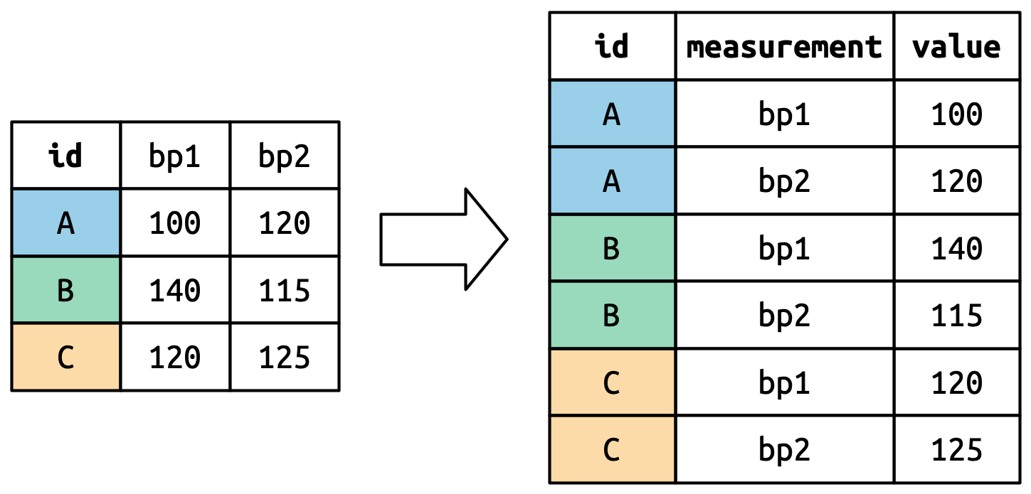
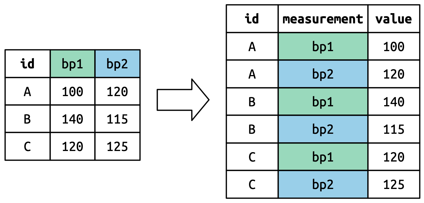
pivot_longer() as it sounds takes a table and breaks down the columns into groups of rows, so in a way we take a short and wide table and transform it into a narrower and longer table. Here are a couple of pictures that graphically explain it:

Let’s think about it column by column. The values in a column that was already a variable in the original dataset (id) need to be repeated, once for each column that’s pivoted. Since we are pivoting one column then it is repeated once. Also, note that the column names (bp1, bp2) become values with the values_to= "value" in a new variable created with the names_to()= measurement column, as shown in the image below

Small dataset
Suppose we have three patients with ids A, B, and C, and we take two blood pressure measurements on each patient. We’ll create the data with tribble(), a handy function for constructing small tibbles by hand:
df <- tribble(
  ~id,  ~bp1, ~bp2,
   "A",  100,  120,
   "B",  140,  115,
   "C",  120,  125
)
We want our new dataset to have three variables: id (already exists), measurement (the column names), and value (the cell values). To achieve this, we need to pivot df longer:
df |>
  pivot_longer(
    cols = bp1:bp2,
    names_to = "measurement",
    values_to = "value"
  )

A tibble:6 × 3
id measurement value
<chr>   <chr>  <dbl>
A   bp1 100
A   bp2 120
B   bp1 140
B   bp2 115
C   bp1 120
C   bp2 125
Now you see how that works compared to the image above. What if we have many variables in column names?
Much wider
In the event that we have multiple variables crammed into column names, and we want to separate them into new variables?
who2
#> # A tibble: 7,240 × 58
#>   country      year sp_m_014 sp_m_1524 sp_m_2534 sp_m_3544 sp_m_4554
#>   <chr>       <dbl>    <dbl>     <dbl>     <dbl>     <dbl>     <dbl>
#> 1 Afghanistan  1980       NA        NA        NA        NA        NA
#> 2 Afghanistan  1981       NA        NA        NA        NA        NA
#> 3 Afghanistan  1982       NA        NA        NA        NA        NA
#> 4 Afghanistan  1983       NA        NA        NA        NA        NA
#> 5 Afghanistan  1984       NA        NA        NA        NA        NA
#> 6 Afghanistan  1985       NA        NA        NA        NA        NA
#> # ℹ 7,234 more rows
#> # ℹ 51 more variables: sp_m_5564 <dbl>, sp_m_65 <dbl>, sp_f_014 <dbl>, …
The above dataset is collected by the World Health Oraganization about TB, as you can see it is 78 columns wide. Notice that two variables are already shown in “country” and “year”. Usually the CodeBook will provide this information:
Column names are broken down by sp_m_xxx for the 3rd column and on and on
sp/rel/ep are the 3 options there followed by
m/f for male or female followed by
digits to represent the age range: 014 = 0-14, 1254= = 15-24…
So we have, country, year, method used, gender, age
We want to add up the number of patients for each category (count=n)
So think of it this way, we want to divide the dataset in groups/categories and we want to know the (country, year, diagnosis method, gender, age, count)
We use
pivot_longer()with a vector of column names fornames_toand instructors for splitting the original variable names into pieces fornames_sepas well as a column name forvalues_toThere might be times that we’ll use
names_patterninstead ofnames_sepfor more complicated splitting of variables
who2 |>
  pivot_longer(
    cols = !(country:year),
    names_to = c("diagnosis", "gender", "age"),
    names_sep = "_",
    values_to = "count"
  )
#> # A tibble: 405,440 × 6
#>   country      year diagnosis gender age   count
#>   <chr>       <dbl> <chr>     <chr>  <chr> <dbl>
#> 1 Afghanistan  1980 sp        m      014      NA
#> 2 Afghanistan  1980 sp        m      1524     NA
#> 3 Afghanistan  1980 sp        m      2534     NA
#> 4 Afghanistan  1980 sp        m      3544     NA
#> 5 Afghanistan  1980 sp        m      4554     NA
#> 6 Afghanistan  1980 sp        m      5564     NA
#> # ℹ 405,434 more rows
Complex headers
The next step up in complexity is when the column names include a mix of variable values and variable names. For example, take the household dataset:
household
#> # A tibble: 5 × 5
#>   family dob_child1 dob_child2 name_child1 name_child2
#>    <int> <date>     <date>     <chr>       <chr>
#> 1      1 1998-11-26 2000-01-29 Susan       Jose
#> 2      2 1996-06-22 NA         Mark        <NA>
#> 3      3 2002-07-11 2004-04-05 Sam         Seth
#> 4      4 2004-10-10 2009-08-27 Craig       Khai
#> 5      5 2000-12-05 2005-02-28 Parker      Gracie
This dataset contains data about five families, with the names and dates of birth of up to two children. The new challenge in this dataset is that
The column names contain the names of two variables (
dob,name) andThe values of another (
child, with values 1 or 2).
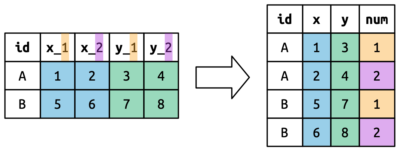
To solve this problem we again need to supply a vector to names_to but this time we use the special ".value" sentinel; this isn’t the name of a variable but a unique value that tells pivot_longer() to do something different. This overrides the usual values_to argument to use the first component of the pivoted column name as a variable name in the output.
We use values_drop_na = TRUE, since the shape of the input forces the creation of explicit missing variables (e.g., for families with only one child).
household |>
  pivot_longer(
    cols = !family,
    names_to = c(".value", "child"),
    names_sep = "_",
    values_drop_na = TRUE
  )
#> # A tibble: 9 × 4
#>   family child  dob        name
#>    <int> <chr>  <date>     <chr>
#> 1      1 child1 1998-11-26 Susan
#> 2      1 child2 2000-01-29 Jose
#> 3      2 child1 1996-06-22 Mark
#> 4      3 child1 2002-07-11 Sam
#> 5      3 child2 2004-04-05 Seth
#> 6      4 child1 2004-10-10 Craig
#> # ℹ 3 more rows
.value
The basic idea of .value is illustrated below. When you use .value in names_to, the column names in the input contribute to both values and variable names in the output using the names_sep for the separation.

Pivot wider
Makes datasets wider by increasing columns and reducing rows and helps when one observation is spread across multiple rows. This seems to arise less commonly, but it does seem to crop up a lot when dealing with governmental data.
We’ll start by looking at cms_patient_experience, a dataset from the Centers of Medicare and Medicaid services that collects data about patient experiences:
cms_patient_experience
#> # A tibble: 500 × 5
#>   org_pac_id org_nm                     measure_cd   measure_title   prf_rate
#>   <chr>      <chr>                      <chr>        <chr>              <dbl>
#> 1 0446157747 USC CARE MEDICAL GROUP INC CAHPS_GRP_1  CAHPS for MIPS…       63
#> 2 0446157747 USC CARE MEDICAL GROUP INC CAHPS_GRP_2  CAHPS for MIPS…       87
#> 3 0446157747 USC CARE MEDICAL GROUP INC CAHPS_GRP_3  CAHPS for MIPS…       86
#> 4 0446157747 USC CARE MEDICAL GROUP INC CAHPS_GRP_5  CAHPS for MIPS…       57
#> 5 0446157747 USC CARE MEDICAL GROUP INC CAHPS_GRP_8  CAHPS for MIPS…       85
#> 6 0446157747 USC CARE MEDICAL GROUP INC CAHPS_GRP_12 CAHPS for MIPS…       24
#> # ℹ 494 more rows
The core unit being studied is an organization, but each organization is spread across six rows, with one row for each measurement taken in the survey organization. We can see the complete set of values for measure_cd and measure_title by using distinct():
cms_patient_experience |>
  distinct(measure_cd, measure_title)
#> # A tibble: 6 × 2
#>   measure_cd   measure_title
#>   <chr>        <chr>
#> 1 CAHPS_GRP_1  CAHPS for MIPS SSM: Getting Timely Care, Appointments, and In…
#> 2 CAHPS_GRP_2  CAHPS for MIPS SSM: How Well Providers Communicate
#> 3 CAHPS_GRP_3  CAHPS for MIPS SSM: Patient's Rating of Provider
#> 4 CAHPS_GRP_5  CAHPS for MIPS SSM: Health Promotion and Education
#> 5 CAHPS_GRP_8  CAHPS for MIPS SSM: Courteous and Helpful Office Staff
#> 6 CAHPS_GRP_12 CAHPS for MIPS SSM: Stewardship of Patient Resources
Neither of these columns will make particularly great variable names: measure_cd doesn’t hint at the meaning of the variable and measure_title is a long sentence containing spaces. We’ll use measure_cd as the source for our new column names for now, but in a real analysis you might want to create your own variable names that are both short and meaningful.
pivot_wider() has the opposite interface to pivot_longer(): instead of choosing new column names, we need to provide the existing columns that define the values (
values_from = prf_rate) and the column name (names_from = measure_cd)
Before we go on, remember the whole idea with lengthening or widening, we basically are grouping, and so far, we have not given R anything that tells it how to group the measure_cd, but let’s do this step anyways:
cms_patient_experience |>
  pivot_wider(
    names_from = measure_cd,
    values_from = prf_rate
  )
#> # A tibble: 500 × 9
#>   org_pac_id org_nm                   measure_title   CAHPS_GRP_1 CAHPS_GRP_2
#>   <chr>      <chr>                    <chr>                 <dbl>       <dbl>
#> 1 0446157747 USC CARE MEDICAL GROUP … CAHPS for MIPS…          63          NA
#> 2 0446157747 USC CARE MEDICAL GROUP … CAHPS for MIPS…          NA          87
#> 3 0446157747 USC CARE MEDICAL GROUP … CAHPS for MIPS…          NA          NA
#> 4 0446157747 USC CARE MEDICAL GROUP … CAHPS for MIPS…          NA          NA
#> 5 0446157747 USC CARE MEDICAL GROUP … CAHPS for MIPS…          NA          NA
#> 6 0446157747 USC CARE MEDICAL GROUP … CAHPS for MIPS…          NA          NA
#> # ℹ 494 more rows
#> # ℹ 4 more variables: CAHPS_GRP_3 <dbl>, CAHPS_GRP_5 <dbl>, …
Ok, so you see we still have multiple rows of the same organization, so let’s see what distinguishes each organization from the other, let’s look in the columns and see if one exists, well if you look at the first two columns, they both start with org_
From tidyr documents:
- id_cols
<
tidy-select> A set of columns that uniquely identify each observation. Typically used when you have redundant variables, i.e. variables whose values are perfectly correlated with existing variables.Defaults to all columns in
dataexcept for the columns specified throughnames_fromandvalues_from. If a tidyselect expression is supplied, it will be evaluated ondataafter removing the columns specified throughnames_fromandvalues_from.
So, let’s assign value to the argument
cms_patient_experience |>
  pivot_wider(
    id_cols = starts_with("org"),
    names_from = measure_cd,
    values_from = prf_rate
  )
#> # A tibble: 95 × 8
#>   org_pac_id org_nm           CAHPS_GRP_1 CAHPS_GRP_2 CAHPS_GRP_3 CAHPS_GRP_5
#>   <chr>      <chr>                  <dbl>       <dbl>       <dbl>       <dbl>
#> 1 0446157747 USC CARE MEDICA…          63          87          86          57
#> 2 0446162697 ASSOCIATION OF …          59          85          83          63
#> 3 0547164295 BEAVER MEDICAL …          49          NA          75          44
#> 4 0749333730 CAPE PHYSICIANS…          67          84          85          65
#> 5 0840104360 ALLIANCE PHYSIC…          66          87          87          64
#> 6 0840109864 REX HOSPITAL INC          73          87          84          67
#> # ℹ 89 more rows
#> # ℹ 2 more variables: CAHPS_GRP_8 <dbl>, CAHPS_GRP_12 <dbl>
The rest of the section will cover examples of actual case studies pertaining to Tidying Data.